Normal Distribution Problems with Solutions
Problems and applications on normal distributions are presented. The solutions to these problems are at the bottom of the page. An online normal probability calculator and an inverse normal probability calculator may be useful to check your answers.

Problems with Solutions
- X is a normally distributed variable with mean = 30 and standard deviation = 4. Find the probabilities a) P(X < 40) b) P(X > 21) c) P(30 < X < 35)
- A radar unit is used to measure the speeds of cars on a motorway. The speeds are normally distributed with a mean of 90 km/hr and a standard deviation of 10 km/hr. What is the probability that a car picked at random is traveling at more than 100 km/hr?
- For certain types of computers, the length of time between charges of the battery is normally distributed with a mean of 50 hours and a standard deviation of 15 hours. John owns one of these computers and wants to know the probability that the length of time will be between 50 and 70 hours.
- Entry to a certain University is determined by a national test. The scores on this test are normally distributed with a mean of 500 and a standard deviation of 100. Tom wants to be admitted to this university and he knows that he must score better than at least 70% of the students who took the test. Tom takes the test and scores 585. Will he be admitted to this university?
- The length of similar components produced by a company is approximated by a normal distribution model with a mean of 5 cm and a standard deviation of 0.02 cm. If a component is chosen at random a) what is the probability that the length of this component is between 4.98 and 5.02 cm? b) What is the probability that the length of this component is between 4.96 and 5.04 cm?
- The length of life of an instrument produced by a machine has a normal distribution with a mean of 12 months and a standard deviation of 2 months. Find the probability that an instrument produced by this machine will last a) less than 7 months. b) between 7 and 12 months.
- The time taken to assemble a car in a certain plant is a random variable having a normal distribution of 20 hours and a standard deviation of 2 hours. What is the probability that a car can be assembled at this plant in a period of time a) less than 19.5 hours? b) between 20 and 22 hours?
- A large group of students took a test in Physics and the final grades have a mean of 70 and a standard deviation of 10. If we can approximate the distribution of these grades by a normal distribution, what percent of the students a) scored higher than 80? b) Should pass the test (grades60)? c) Should fail the test (grades<60)?
- The annual salaries of employees in a large company are approximately normally distributed with a mean of $50,000 and a standard deviation of $20,000. a) What percent of people earn less than $40,000? b) What percent of people earn between $45,000 and $65,000? c) What percent of people earn more than $70,000?
Solutions to the Above Problems
- Note: What is meant here by area is the area under the standard normal curve. a) For x = 40, the z-value z = (40 - 30) / 4 = 2.5 Hence P(x < 40) = P(z < 2.5) = [area to the left of 2.5] = 0.9938 b) For x = 21, z = (21 - 30) / 4 = -2.25 Hence P(x > 21) = P(z > -2.25) = [total area] - [area to the left of -2.25] = 1 - 0.0122 = 0.9878 c) For x = 30 , z = (30 - 30) / 4 = 0 and for x = 35, z = (35 - 30) / 4 = 1.25 Hence P(30 < x < 35) = P(0 < z < 1.25) = [area to the left of z = 1.25] - [area to the left of 0] = 0.8944 - 0.5 = 0.3944
- Let x be the random variable that represents the speed of cars. x has = 90 and = 10. We have to find the probability that x is higher than 100 or P(x > 100) For x = 100 , z = (100 - 90) / 10 = 1 P(x > 90) = P(z > 1) = [total area] - [area to the left of z = 1] = 1 - 0.8413 = 0.1587 The probability that a car selected at random has a speed greater than 100 km/hr is equal to 0.1587
- Let x be the random variable that represents the length of time. It has a mean of 50 and a standard deviation of 15. We have to find the probability that x is between 50 and 70 or P( 50< x < 70) For x = 50 , z = (50 - 50) / 15 = 0 For x = 70 , z = (70 - 50) / 15 = 1.33 (rounded to 2 decimal places) P( 50< x < 70) = P( 0< z < 1.33) = [area to the left of z = 1.33] - [area to the left of z = 0] = 0.9082 - 0.5 = 0.4082 The probability that John's computer has a length of time between 50 and 70 hours is equal to 0.4082.
- Let x be the random variable that represents the scores. x is normally distributed with a mean of 500 and a standard deviation of 100. The total area under the normal curve represents the total number of students who took the test. If we multiply the values of the areas under the curve by 100, we obtain percentages. For x = 585 , z = (585 - 500) / 100 = 0.85 The proportion P of students who scored below 585 is given by P = [area to the left of z = 0.85] = 0.8023 = 80.23% Tom scored better than 80.23% of the students who took the test and he will be admitted to this University.
- a) P(4.98 < x < 5.02) = P(-1 < z < 1) = 0.6826 b) P(4.96 < x < 5.04) = P(-2 < z < 2) = 0.9544
- a) P(x < 7) = P(z < -2.5) = 0.0062 b) P(7 < x < 12) = P(-2.5 < z < 0) = 0.4938
- a) P(x < 19.5) = P(z < -0.25) = 0.4013 b) P(20 < x < 22) = P(0 < z < 1) = 0.3413
- a) For x = 80, z = 1 Area to the right (higher than) z = 1 is equal to 0.1586 = 15.87% scored more that 80. b) For x = 60, z = -1 The area to the right of z = -1 is equal to 0.8413 = 84.13% should pass the test. c) 100% - 84.13% = 15.87% should fail the test.
- a) For x = 40000, z = -0.5 The area to the left (less than) of z = -0.5 is equal to 0.3085 = 30.85% earn less than $40,000. b) For x = 45000 , z = -0.25 and for x = 65000, z = 0.75 The area between z = -0.25 and z = 0.75 is equal to 0.3720 = 37.20 earning between $45,000 and $65,000. c) For x = 70000, z = 1 The area to the right (higher) of z = 1 is equal to 0.1586 = 15.86% earning more than $70,000.
More References and links
- Normal Distribution Definition
- Elementary statistics and probabilities
Lesson 16: Normal Distributions
In this lesson, we'll investigate one of the most prevalent probability distributions in the natural world, namely the normal distribution . Just as we have for other probability distributions, we'll explore the normal distribution's properties, as well as learn how to calculate normal probabilities.
- To define the probability density function of a normal random variable.
- To learn the characteristics of a typical normal curve.
- To learn how to transform a normal random variable \(X\) into the standard normal random variable \(Z\).
- To learn how to calculate the probability that a normal random variable \(X\) falls between two values \(a\) and \(b\) , below a value \(c\), or above a value \(d\) .
- To learn how to read standard normal probability tables.
- To learn how to find the value \(x\) associated with a cumulative normal probability.
- To explore the key properties, such as the moment-generating function, mean and variance, of a normal random variable.
- To investigate the relationship between the standard normal random variable and a chi-square random variable with one degree of freedom.
- To learn how to interpret a \(Z\)-value.
- To learn why the Empirical Rule holds true.
- To understand the steps involved in each of the proofs in the lesson.
- To be able to apply the methods learned in the lesson to new problems.
16.1 - The Distribution and Its Characteristics
The continuous random variable \(X\) follows a normal distribution if its probability density function is defined as:
\(f(x)=\dfrac{1}{\sigma \sqrt{2\pi}} \text{exp}\left\{-\dfrac{1}{2} \left(\dfrac{x-\mu}{\sigma}\right)^2\right\}\)
for \(-\infty<x<\infty\), \(-\infty<\mu<\infty\), and \(0<\sigma<\infty\). The mean of \(X\) is \(\mu\) and the variance of \(X\) is \(\sigma^2\). We say \(X\sim N(\mu, \sigma^2)\).
With a first exposure to the normal distribution, the probability density function in its own right is probably not particularly enlightening. Let's take a look at an example of a normal curve, and then follow the example with a list of the characteristics of a typical normal curve.
Example 16-1
Let \(X\) denote the IQ (as determined by the Stanford-Binet Intelligence Quotient Test) of a randomly selected American. It has long been known that \(X\) follows a normal distribution with mean 100 and standard deviation of 16. That is, \(X\sim N(100, 16^2)\). Draw a picture of the normal curve, that is, the distribution, of \(X\).
Note that when drawing the above curve, I said "now what a standard normal curve looks like... it looks something like this." It turns out that the term " standard normal curve " actually has a specific meaning in the study of probability. As we'll soon see, it represents the case in which the mean \(\mu\) equals 0 and the standard deviation σ equals 1. So as not to cause confusion, I wish I had said "now what a typical normal curve looks like...." Anyway, on to the characteristics of all normal curves!
Characteristics of a Normal Curve
It is the following known characteristics of the normal curve that directed me in drawing the curve as I did so above.
All normal curves are bell-shaped with points of inflection at \(\mu\pm \sigma\).
The proof is left for you as an exercise
All normal curves are symmetric about the mean \(\mu\) .
All normal curves are symmetric about the mean \(\mu\), because \(f(\mu+x)=f(\mu-x)\) for all \(x\). That is:
\(f(\mu+x)=\dfrac{1}{\sigma \sqrt{2\pi}} \text{exp}\left\{-\dfrac{1}{2} \left(\dfrac{x+\mu-\mu}{\sigma}\right)^2\right\} =\dfrac{1}{\sigma \sqrt{2\pi}} \text{exp}\left\{-\dfrac{1}{2} \left(\dfrac{x}{\sigma}\right)^2\right\}\)
\(f(\mu-x)=\dfrac{1}{\sigma \sqrt{2\pi}} \text{exp}\left\{-\dfrac{1}{2} \left(\dfrac{\mu-x-\mu}{\sigma}\right)^2\right\} =\dfrac{1}{\sigma \sqrt{2\pi}} \text{exp}\left\{-\dfrac{1}{2} \left(\dfrac{-x}{\sigma}\right)^2\right\}=\dfrac{1}{\sigma \sqrt{2\pi}} \text{exp}\left\{-\dfrac{1}{2} \left(\dfrac{x}{\sigma}\right)^2\right\}\)
Therefore, by the definition of symmetry, the normal curve is symmetric about the mean \(\mu\).
The area under an entire normal curve is 1.
All normal curves are positive for all \(x\). That is, \(f(x)>0\) for all \(x\).
The standard deviation \(\sigma\) is defined to be positive. The square root of \(2\pi\) is positive. And, the natural exponential function is positive. When you multiply positive terms together, you, of course, get a positive number.
The limit of \(f(x)\) as \(x\) goes to infinity is 0, and the limit of \(f(x)\) as \(x\) goes to negative infinity is 0. That is:
\(\lim\limits_{x\to \infty} f(x)=0\) and \(\lim\limits_{x\to -\infty} f(x)=0\)
The function \(f(x)\) depends on \(x\) only through the natural exponential function \(\exp[-x^2]\), which is known to approach 0 as \(x\) approaches infinity or negative infinity.
The height of any normal curve is maximized at \(x=\mu\).
Using what we know from our calculus studies, to find the point at which the maximum occurs, we must differentiate \(f(x)\) with respect to \(x\) and solve for \(x\) to find the maximum. Because our \(f(x)\) contains the natural exponential function, however, it is easier to take the derivative of the natural log of \(f(x)\) with respect to \(x\) and solve for \(x\) to find the maximum. [The maximum of \(f(x)\) is the same as the maximum of the natural log of \(f(x)\), because \(\log_e(x)\) is an increasing function of \(x\). That is, \(x_1<x_2\) implies that \(\log_e(x_1)<\log_e(x_2)\). Therefore, \(f(x_1)<f(x_2)\) implies \(\log_e(f(x_1))<\log_e(f(x_2))\).] That said, taking the natural log of \(f(x)\), we get:
\(\text{log}_e (f(x))=\text{log}\left(\dfrac{1}{\sigma \sqrt{2\pi}} \right)-\dfrac{1}{2\sigma^2}(x-\mu)^2\)
Taking the derivative of \(\log_e(f(x))\) with respect to \(x\), we get:
\(\dfrac{d\text{log}f(x)}{dx}=-\dfrac{1}{2\sigma^2}\cdot 2(x-\mu)\)
Now, setting the derivative of \(\log_e(f(x))\) to 0:
\(\dfrac{d\text{log}f(x)}{dx}=-\dfrac{1}{2\sigma^2}\cdot 2(x-\mu) \stackrel{\equiv}{\scriptscriptstyle{SET}} 0\)
and solving for \(x\), we get that \(x=\mu\). Taking the second derivative of \(\log_e(f(x))\) with respect to \(x\), we get:
\(\dfrac{d^2\text{log}f(x)}{dx^2}=-\dfrac{1}{\sigma^2}\)
Because the second derivative of \(\log_e(f(x))\) is negative (for all \(x\), in fact), the point \(x=\mu\) is deemed a local maximum.
The shape of any normal curve depends on its mean \(\mu\) and standard deviation \(\sigma\).
Given that the curve \(f(x)\) depends only on \(x\) and the two parameters \(\mu\) and \(\sigma\), the claimed characteristic is quite obvious. An example is perhaps more interesting than the proof. Here is a picture of three superimposed normal curves —one of a \(N(0,9)\) curve, one of a \(N(0, 16)\) curve, and one of a \(N(1, 9)\) curve:
As claimed, the shapes of the three curves differ, as the means \(\mu\) and standard deviations \(\sigma\) differ.
16.2 - Finding Normal Probabilities
Example 16-2.
Let \(X\) equal the IQ of a randomly selected American. Assume \(X\sim N(100, 16^2)\). What is the probability that a randomly selected American has an IQ below 90?
As is the case with all continuous distributions, finding the probability involves finding the area under the curve and to the left of the line \(x=90\):
\(P(X \leq 90)=F(90)=\int^{90}_{-\infty} \dfrac{1}{16\sqrt{2\pi}}\text{exp}\left\{-\dfrac{1}{2}\left(\dfrac{x-100}{16}\right)^2\right\} dx\)
There's just one problem... it is not possible to integrate the normal p.d.f. That is, no simple expression exists for the antiderivative. We can only approximate the integral using numerical analysis techniques. So, all we need to do is find a normal probability table for a normal distribution with mean \(\mu=100\) and standard deviation \(\sigma=16\). Aw, geez, there'd have to be an infinite number of normal probability tables. That strategy isn't going to work! Aha! The cumulative probabilities have been tabled for the \(N(0,1)\) distribution. All we need to do is transform our \(N(100, 16^2)\) distribution to a \(N(0, 1)\) distribution and then use the cumulative probability table for the \(N(0,1)\) distribution to calculate our desired probability. The theorem that follows tells us how to make the necessary transformation.
If \(X\sim N(\mu, \sigma^2)\), then:
\(Z=\dfrac{X-\mu}{\sigma}\)
follows the \(N(0,1)\) distribution, which is called the standardized (or standard ) normal distribution .
We need to show that the random variable \(Z\) follows a \(N(0,1)\) distribution. So, let's find the cumulative distribution function \(F(z)\), which is also incidentally referred to as \(\Phi(z)\) in the standard normal case (that's the greek letter phi, read "fee"):
\(F(z)=\Phi(z)=P(Z\leq z)=P \left(\dfrac{X-\mu}{\sigma} \leq z \right)\)
which, by rearranging and using the normal p.d.f., equals:
\(F(z)=P(X\leq \mu+z\sigma)=\int^{\mu+z\sigma}_{-\infty} \dfrac{1}{\sigma \sqrt{2\pi}} \text{exp}\left\{-\dfrac{1}{2} \left(\dfrac{x-\mu}{\sigma}\right)^2\right\} \)
To perform the integration, let's use the change of variable technique with:
\(w=\dfrac{x-\mu}{\sigma}\)
\(x = \sigma(w) + \mu \) and \(dx = \sigma dw\)
Now for the endpoints of the integral: if \(x=-\infty\), then \(w\) also equals \(-\infty\); and if \(x=\mu+z\sigma\), then \(w=\frac{\mu+z\sigma -\mu}{\sigma}\). Therefore, upon making all of the substitutions for \(x, w\), and \(dx\), our integration looks like this:
\(F(z)=\int^z_{-\infty}\dfrac{1}{\sigma \sqrt{2\pi}} \text{exp}\left\{-\dfrac{1}{2} w^2\right\} \sigma dw\)
And since the \(\sigma\) in the denominator cancels out the \(\sigma\) in the numerator, we get:
\(F(z)=\int^z_{-\infty}\dfrac{1}{\sqrt{2\pi}} \text{exp}\left\{-\dfrac{1}{2} w^2\right\} dw\)
We should now recognize that as the cumulative distribution of a normal random variable with mean \(\mu=0\) and standard deviation \(\sigma=1\). Our proof is complete.
The theorem leads us to the following strategy for finding probabilities \(P(z<X<b)\) when \(a\) and \(b\) are constants, and \(X\) is a normal random variable with mean \(\mu\) and standard deviation \(\sigma\):
1) Specify the desired probability in terms of \(X\).
2) Transform \(X, a\), and \(b\), by:
3) Use the standard normal \(N(0,1)\) table, typically referred to as the \(Z\) -table , to find the desired probability.
Reading \(Z\)-tables
Standard normal, or \(Z\)-tables, can take a number of different forms. There are two standard normal tables, Table Va and Table Vb, in the back of our textbook. Table Va gives the cumulative probabilities for \(Z\)-values, to two decimal places, between 0.00 and 3.09. Here's what the top of Table Va looks like:
\begin{aligned} P(Z \leq z)=& \Phi(z)=\int_{-\infty}^{z} \frac{1}{\sqrt{2 \pi}} e^{-w^{2} / 2} d w \\ \Phi(-z) &=1-\Phi(z) \end{aligned}
For example, you could use Table Va to find probabilities such as \(P(Z\le 0.01), P(Z\le 1.23)\), or \(P(Z\le 2.98)\). Table Vb , on the other hand, gives probabilities in the upper tail of the standard normal distribution. Here's what the top of Table Vb looks like:
\(P(Z > z_\alpha) = \alpha \)
\(P(Z > z) = 1 - \Phi(z) = \Phi(-z)\)
That is, for \(Z\)-values, to two decimal places, between 0.00 and 3.49, we can use Table Vb to find probabilities such as \(P(Z>0.12), P(Z>1.96)\), and \(P(Z>3.32)\).
Now, we just need to learn how to read the probabilities off of each of the tables. First Table Va:
And, then Table Vb:
Now we know how to read the given \(Z\)-tables. Now, we just need to work with some real examples to see that finding probabilities associated with a normal random variable usually involves rewriting the problems just a bit in order to get them to "fit" with the available \(Z\)-tables.
Example 16-2 Continued
Whenever I am faced with finding a normal probability, I always always always draw a picture of the probability I am trying to find. Then, the problem usually just solves itself... oh, how we wish:
So, we just found that the desired probability, that is, that the probability that a randomly selected American has an IQ below 90 is 0.2643. (If you haven't already, you might want to make sure that you can independently read that probability off of Table Vb.)
Now, although I used Table Vb in finding our desired probability, it is worth mentioning that I could have alternatively used Table Va. How's that? Well:
\(P(X<90)=P(Z<-0.63)=P(Z>0.63)=1-P(Z<0.63)\)
where the first equality comes from the transformation from \(X\) to \(Z\), the second equality comes from the symmetry of the normal distribution, and the third equality comes from the rule of complementary events. Using Table Va to look up \(P(Z<0.63)\), we get 0.7357. Therefore,
\(P(X<90)=1-P(Z<0.63)=1-0.7357=0.2643\)
We should, of course, be reassured that our logic produced the same answer regardless of the method used! That's always a good thing!
What is the probability that a randomly selected American has an IQ above 140?
Again, I am going to solve this problem by drawing a picture:
So, we just found that the desired probability, that is, that the probability that a randomly selected American has an IQ above 140 is 0.0062. (Again, if you haven't already, you might want to make sure that you can independently read that probability off of Table Vb.)
We again could have alternatively used Table Va to find our desired probability:
\(P(X>140)=P(Z>2.50)=1-P(Z<2.50\)
where the first equality comes from the transformation from \(X\) to \(Z\), and the second equality comes from the rule of complementary events. Using Table Va to look up \(P(Z<2.5)\), we get 0.9938. Therefore,
\(P(X>140)=1-P(Z<2.50)=1-0.9938=0.0062\)
Again, we arrived at the same answer using two different methods.
What is the probability that a randomly selected American has an IQ between 92 and 114?
So, we just found that the desired probability, that is, that the probability that a randomly selected American has an IQ between 92 and 114 is 0.5021. (Again, if you haven't already, you might want to make sure that you can independently read the probabilities that we used to get the answer from Tables Va and Vb.)
The previous three examples have illustrated each of the three possible normal probabilities you could be faced with finding —below some number, above some number, and between two numbers. Once you have mastered each case, then you should be able to find any normal probability when asked.
16.3 - Using Normal Probabilities to Find X
On the last page, we learned how to use the standard normal curve N (0, 1) to find probabilities concerning a normal random variable X with mean \(\mu\) and standard deviation \(\sigma\). What happens if it's not the probability that we want to find, but rather the value of X ? That's what we'll investigate on this page. That is, we'll consider what I like to call "inside-out" problems, in which we use known probabilities to find the value of the normal random variable X . Let's start with an example.
Example 16-3
Suppose X , the grade on a midterm exam, is normally distributed with mean 70 and standard deviation 10. The instructor wants to give 15% of the class an A. What cutoff should the instructor use to determine who gets an A?
My approach to solving this problem is, of course, going to involve drawing a picture:
The instructor now wants to give 10% of the class an A−. What cutoff should the instructor use to determine who gets an A−?
We'll use the same method as we did previously:
In summary, in order to use a normal probability to find the value of a normal random variable X :
Find the z value associated with the normal probability.
Use the transformation \(x = \mu + z \sigma\) to find the value of x .
16.4 - Normal Properties
So far, all of our attention has been focused on learning how to use the normal distribution to answer some practical problems. We'll turn our attention for a bit to some of the theoretical properties of the normal distribution. We'll start by verifying that the normal p.d.f. is indeed a valid probability distribution. Then, we'll derive the moment-generating function \(M(t)\) of a normal random variable \(X\). We'll conclude by using the moment generating function to prove that the mean and standard deviation of a normal random variable \(X\) are indeed, respectively, \(\mu\) and \(\sigma\), something that we thus far have assumed without proof.
The Normal P.D.F. is Valid
Recall that the probability density function of a normal random variable is:
for \(-\infty<x<\infty\), \(-\infty<\mu<\infty\), and \(0<\sigma<\infty\). Also recall that in order to show that the normal p.d.f. is a valid p.d.f, we need to show that, firstly \(f(x)\) is always positive, and, secondly, if we integrate \(f(x)\) over the entire support, we get 1.
Let's start with the easy part first, namely, showing that \(f(x)\) is always positive. The standard deviation \(\sigma\) is defined to be positive. The square root of \(2\pi\) is positive. And, the natural exponential function is positive. When you multiply positive terms together, you, of course, get a positive number. Check... the first part is done.
Now, for the second part. Showing that \(f(x)\) integrates to 1 is a bit messy, so bear with me here. Let's define \(I\) to be the integral that we are trying to find. That is:
\(I=\int_{-\infty}^\infty \dfrac{1}{\sigma \sqrt{2\pi}} \text{exp}\left\{-\dfrac{1}{2\sigma^2} (x-\mu)^2\right\}dx\)
Our goal is to show that \(I=1\). Now, if we change variables with:
our integral \(I\) becomes:
\(I=\int_{-\infty}^\infty \dfrac{1}{\sqrt{2\pi}} \text{exp}\left\{-\dfrac{1}{2} w^2\right\}dw\)
Now, squaring both sides, we get:
\(I^2=\left(\int_{-\infty}^\infty \dfrac{1}{\sqrt{2\pi}} \text{exp}\left\{-\dfrac{x^2}{2} \right\}dx\right) \left(\int_{-\infty}^\infty \dfrac{1}{\sqrt{2\pi}} \text{exp}\left\{-\dfrac{y^2}{2} \right\}dy\right)\)
And, pulling the integrals together, we get:
\(I^2=\dfrac{1}{2\pi}\int_{-\infty}^\infty \int_{-\infty}^\infty \text{exp}\left\{-\dfrac{x^2}{2} \right\} \text{exp}\left\{-\dfrac{y^2}{2} \right\}dxdy\)
Now, combining the exponents, we get:
\(I^2=\dfrac{1}{2\pi}\int_{-\infty}^\infty \int_{-\infty}^\infty \text{exp}\left\{-\dfrac{1}{2}(x^2+y^2) \right\} dxdy\)
Converting to polar coordinates with:
\(x=r\cos\theta\) and \(y=r\sin\theta\)
\(I^2=\dfrac{1}{2\pi}\int_0^{2\pi}\left(\int_0^\infty \text{exp}\left\{-\dfrac{r^2}{2} \right\} rdr\right)d\theta \)
Now, if we do yet another change of variables with:
\(u=\dfrac{r^2}{2}\) and \(du=rdr\)
\(I^2=\dfrac{1}{2\pi}\int_0^{2\pi}\left(\int_0^\infty e^{-u}du\right)d\theta \)
Evaluating the inside integral, we get:
\(I^2=\dfrac{1}{2\pi}\int_0^{2\pi}\left\{-\lim\limits_{b\to \infty} [e^{-u}]^{u=b}_{u=0}\right\}d\theta \)
And, finally, completing the integration, we get:
\(I^2=\dfrac{1}{2\pi} \int_0^{2\pi} -(0-1) d \theta= \dfrac{1}{2\pi}\int_0^{2\pi} d \theta =\dfrac{1}{2\pi} (2\pi)=1\)
Okay, so we've shown that \(I^2=1\). Therefore, that means that \(I=+1\) or \(I=-1\). But, we know that \(I\) must be positive, since \(f(x)>0\). Therefore, \(I\) must equal 1. Our proof is complete. Finally.
The Moment Generating Function
The moment generating function of a normal random variable \(X\) is:
\(M(t)=\text{exp}\left\{\mu t+\dfrac{\sigma^2 t^2}{2}\right\}\)
Well, I better start this proof out by saying this one is a bit messy, too. Jumping right into it, using the definition of a moment-generating function, we get:
\(M(t)=E(e^{tX})=\int_{-\infty}^\infty e^{tx}f(x)dx=\int_{-\infty}^\infty e^{tx}\left[\dfrac{1}{\sigma \sqrt{2\pi}} \text{exp}\left\{-\dfrac{1}{2\sigma^2} (x-\mu)^2\right\} \right]dx\)
Simply expanding the term in the second exponent, we get:
\(M(t)=\int_{-\infty}^\infty \dfrac{1}{\sigma \sqrt{2\pi}}\text{exp}\{tx\} \text{exp}\left\{-\dfrac{1}{2\sigma^2} (x^2-2x\mu+\mu^2)\right\} dx\)
And, combining the two exponents, we get:
\(M(t)=\int_{-\infty}^\infty \dfrac{1}{\sigma \sqrt{2\pi}} \text{exp}\left\{-\dfrac{1}{2\sigma^2} (x^2-2x\mu+\mu^2)+tx \right\} dx\)
Pulling the \(tx\) term into the parentheses in the exponent, we get:
\(M(t)=\int_{-\infty}^\infty \dfrac{1}{\sigma \sqrt{2\pi}} \text{exp}\left\{-\dfrac{1}{2\sigma^2} (x^2-2x\mu-2\sigma^2tx+\mu^2) \right\} dx\)
And, simplifying just a bit more in the exponent, we get:
\(M(t)=\int_{-\infty}^\infty \dfrac{1}{\sigma \sqrt{2\pi}} \text{exp}\left\{-\dfrac{1}{2\sigma^2} (x^2-2x(\mu+\sigma^2 t)+\mu^2) \right\} dx\)
Now, let's take a little bit of an aside by focusing our attention on just this part of the exponent:
\((x^2-2(\mu+\sigma^2t)x+\mu^2)\)
\(a=\mu+\sigma^2t\) and \(b=\mu^2\)
then that part of our exponent becomes:
\(x^2-2(\mu+\sigma^2t)x+\mu^2=x^2-2ax+b\)
Now, complete the square by effectively adding 0:
\(x^2-2(\mu+\sigma^2t)x+\mu^2=x^2-2ax+a^2-a^2+b\)
And, simplifying, we get:
\(x^2-2(\mu+\sigma^2t)x+\mu^2=(x-a)^2-a^2+b\)
Now, inserting in the values we defined for \(a\) and \(b\), we get:
\(x^2-2(\mu+\sigma^2t)x+\mu^2=(x-(\mu+\sigma^2t))^2-(\mu+\sigma^2t)^2+\mu^2\)
Okay, now stick our modified exponent back into where we left off in our calculation of the moment-generating function:
\(M(t)=\int_{-\infty}^\infty \dfrac{1}{\sigma \sqrt{2\pi}}\text{exp}\left\{-\dfrac{1}{2\sigma^2}\left[(x-(\mu+\sigma^2t))^2-(\mu+\sigma^2t)^2+\mu^2\right]\right\}dx\)
We can now pull the part of the exponent that doesn't depend on \(x\) through the integral getting:
\(M(t)=\text{exp}\left\{-\dfrac{1}{2\sigma^2}\left[-(\mu+\sigma^2t)^2+\mu^2\right]\right\} \int_{-\infty}^\infty \dfrac{1}{\sigma \sqrt{2\pi}}\text{exp}\left\{-\dfrac{1}{2\sigma^2}\left[(x-(\mu+\sigma^2t))^2 \right]\right\}dx\)
Now, we should recognize that the integral integrates to 1 because it is the integral over the entire support of the p.d.f. of a normal random variable \(X\) with:
mean \(\mu+\sigma^2t\) and variance \(\sigma^2\)
That is, because the integral is 1:
\(\int_{-\infty}^\infty \dfrac{1}{\sigma \sqrt{2\pi}}\text{exp}\left\{-\dfrac{1}{2\sigma^2}\left[(x-(\mu+\sigma^2t))^2 \right]\right\}dx = 1\) \(\text{Since, }\ N(\mu+\sigma^2t, \sigma^2)\)
our moment-generating function reduces to this:
\(M(t)=\text{exp}\left\{-\dfrac{1}{2\sigma^2}\left[-\mu^2-2\mu\sigma^2t-\sigma^4t^2+\mu^2\right]\right\}\)
Now, it's just a matter of simplifying:
\(M(t)=\text{exp}\left\{\dfrac{2\mu\sigma^2t+\sigma^4t^2}{2\sigma^2}\right\}\)
and simplifying a bit more:
\(M(t)=\text{exp}\left\{\mu t +\dfrac{\sigma^2t^2}{2}\right\}\)
Our second messy proof is complete!
The Mean and Variance
The mean and variance of a normal random variable \(X\) are, respectively, \(\mu\) and \(\sigma^2\).
We'll use the moment generating function:
to find the mean and variance. Recall that finding the mean involves evaluating the derivative of the moment-generating function with respect to \(t\) at \(t=0\):
So, we just found that the first derivative of the moment-generating function with respect to \(t\) is:
\(M'(t)=\text{exp}\left(\mu t +\dfrac{\sigma^2t^2}{2}\right)\times (\mu+\sigma^2t)\)
We'll use it to help us find the variance:
16.5 - The Standard Normal and The Chi-Square
We have one more theoretical topic to address before getting back to some practical applications on the next page, and that is the relationship between the normal distribution and the chi-square distribution. The following theorem clarifies the relationship.
If \(X\) is normally distributed with mean \(\mu\) and variance \(\sigma^2>0\), then:
\(V=\left(\dfrac{X-\mu}{\sigma}\right)^2=Z^2\)
is distributed as a chi-square random variable with 1 degree of freedom.
To prove this theorem, we need to show that the p.d.f. of the random variable \(V\) is the same as the p.d.f. of a chi-square random variable with 1 degree of freedom. That is, we need to show that:
\(g(v)=\dfrac{1}{\Gamma(1/2)2^{1/2}}v^{\frac{1}{2}-1} e^{-v/2}\)
The strategy we'll take is to find \(G(v)\), the cumulative distribution function of \(V\), and then differentiate it to get \(g(v)\), the probability density function of \(V\). That said, we start with the definition of the cumulative distribution function of \(V\):
\(G(v)=P(V\leq v)=P(Z^2 \leq v)\)
That second equality comes, of course, from the fact that \(V=Z^2\). Now, taking note of the behavior of a parabolic function:
we can simplify \(G(v)\) to get:
\(G(v)=P(-\sqrt{v} < Z <\sqrt{v})\)
Now, to find the desired probability we need to integrate, over the given interval, the probability density function of a standard normal random variable \(Z\). That is:
\(G(v)= \int^{\sqrt{v}}_{-\sqrt{v}}\dfrac{1}{ \sqrt{2\pi}}\text{exp} \left(-\dfrac{z^2}{2}\right) dz\)
By the symmetry of the normal distribution, we can integrate over just the positive portion of the integral, and then multiply by two:
\(G(v)= 2\int^{\sqrt{v}}_0 \dfrac{1}{ \sqrt{2\pi}}\text{exp} \left(-\dfrac{z^2}{2}\right) dz\)
Okay, now let's do the following change of variables:
\(\text{Let}\ z=\sqrt{y}=y^{1/2}\)
\(\text{So, }\ dz=\frac{1}{2}y^{-1/2}\ dy=\frac{1}{z\sqrt{y}}dy\)
\(z^2=y,\ \\ \begin{aligned} z&=0 \Rightarrow y=0 \\ z&=\sqrt{v} \Rightarrow y=v\end{aligned}\)
Doing so, we get:
\(G(v)= 2\int^v_0 \dfrac{1}{ \sqrt{2\pi}}\text{exp} \left(-\dfrac{y}{2}\right) \left(\dfrac{1}{2\sqrt{y}}\right) dy\)
\(G(v)= \int^v_0 \dfrac{1}{ \sqrt{\pi}\sqrt{2}} y^{\frac{1}{2}-1} \text{exp} \left(-\dfrac{y}{2}\right) dy\)
for \(v>0\). Now, by one form of the Fundamental Theorem of Calculus:
\(\text{Given, }\)
\(\int^x_a f(t)dt=F(x)-F(a)\)
\(\frac{d}{dx}\int^x_a f(t)dt=F'(x)=f(x)\)
we can take the derivative of \(G(v)\) to get the probability density function \(g(v)\):
\(g(v)=G'(v)= \dfrac{1}{ \sqrt{\pi}\sqrt{2}} v^{\frac{1}{2}-1} e^{-v/2}\)
for \(0<v<\infty\). If you compare this \(g(v)\) to the first \(g(v)\) that we said we needed to find way back at the beginning of this proof, you should see that we are done if the following is true:
\(\Gamma \left(\dfrac{1}{2}\right)=\sqrt{\pi}\)
It is indeed true, as the following argument illustrates. Because \(g(v)\) is a p.d.f., the integral of the p.d.f. over the support must equal 1:
\(\int_0^\infty \dfrac{1}{ \sqrt{\pi}\sqrt{2}} v^{\frac{1}{2}-1} e^{-v/2} dv=1\)
Now, change the variables by letting \(v=2x\), so that \(dv=2dx\). Making the change, we get:
\(\dfrac{1}{ \sqrt{\pi}} \int_0^\infty \dfrac{1}{ \sqrt{2}} (2x)^{\frac{1}{2}-1} e^{-x}2dx=1\)
Rewriting things just a bit, we get:
\(\dfrac{1}{ \sqrt{\pi}} \int_0^\infty \dfrac{1}{ \sqrt{2}}\dfrac{1}{ \sqrt{2}} x^{\frac{1}{2}-1} e^{-x}2dx=1\)
And simplifying, we get:
\(\dfrac{1}{ \sqrt{\pi}} \int_0^\infty x^{\frac{1}{2}-1} e^{-x} dx=1\)
Now, it's just a matter of recognizing that the integral is the gamma function of \(\frac{1}{2}\):
\(\dfrac{1}{ \sqrt{\pi}} \Gamma \left(\dfrac{1}{2}\right)=1\)
Our proof is complete.
So, now that we've taken care of the theoretical argument. Let's take a look at an example to see that the theorem is, in fact, believable in a practical sense.
Example 16-4
Find the probability that the standard normal random variable \(Z\) falls between −1.96 and 1.96 in two ways:
- using the standard normal distribution
- using the chi-square distribution
The standard normal table (Table V in the textbook) yields:
\(P(-1.96<Z<1.96)=P(Z<1.96)-P(Z>1.96)=0.975-0.025=0.95\)
The chi-square table (Table IV in the textbook) yields the same answer:
\(P(-1.96<Z<1.96)=P(|Z|<1.96)=P(Z^2<1.96^2)=P(\chi^2_{(1)})<3.8416)=0.95\)
16.6 - Some Applications
Interpretation of z.
Note that the transformation from \(X\) to \(Z\):
tells us the number of standard deviations above or below the mean that \(X\) falls. That is, if \(Z=-2\), then we know that \(X\) falls 2 standard deviations below the mean. And if \(Z=+2\), then we know that \(X\) falls 2 standard deviations above the mean. As such, \(Z\)-scores are sometimes used in medical fields to identify whether an individual exhibits extreme values with respect to some biological or physical measurement.
Example 16-5

Post-menopausal women are known to be susceptible to severe bone loss known as osteoporosis. In some cases, bone loss can be so extreme as to cause a woman to lose a few inches of height. The spines and hips of women who are suspected of having osteoporosis are therefore routinely scanned to ensure that their bone loss hasn't become so severe to warrant medical intervention.
The mean \(\mu\) and standard deviation \(\sigma\) of the density of the bones in the spine, for example, are known for a healthy population. A woman is scanned and \(x\), the bone density of her spine is determined. She and her doctor would then naturally want to know whether the woman's bone density \(x\) is extreme enough to warrant medical intervention. The most common way of evaluating whether a particular \(x\) is extreme is to use the mean \(\mu\), the standard deviation \(\sigma\), and the value \(x\) to calculate a \(Z\)-score. The \(Z\)-score can then be converted to a percentile to provide the doctor and the woman an indication of the severity of her bone loss.
Suppose the woman's \(Z\)-score is −2.36, for example. The doctor then knows that the woman's bone density falls 2.36 standard deviations below the average bone density of a healthy population. The doctor, furthermore, knows that fewer than 1% of the population have a bone density more extreme than that of his/her patient.
The Empirical Rule Revisited
You might recall earlier in this section, when we investigated exploring continuous data, that we learned about the Empirical Rule. Specifically, we learned that if a histogram is at least approximately bell-shaped, then:
- approximately 68% of the data fall within one standard deviation of the mean
- approximately 95% of the data fall within two standard deviations of the mean
- approximately 99.7% of the data fall within three standard deviations of the mean
Where did those numbers come from? Now, that we've got the normal distribution under our belt, we can see why the Empirical Rule holds true. The probability that a randomly selected data value from a normal distribution falls within one standard deviation of the mean is
\(P(-1<Z<1)=P(Z<1)-P(Z>1)=0.8413-0.1587=0.6826\)
That is, we should expect 68.26% (approximately 68%!) of the data values arising from a normal population to be within one standard deviation of the mean, that is, to fall in the interval:
\((\mu-\sigma, \mu+\sigma)\)
The probability that a randomly selected data value from a normal distribution falls within two standard deviations of the mean is
\(P(-2<Z<2)=P(Z<2)-P(Z>2)=0.9772-0.0228=0.9544\)
That is, we should expect 95.44% (approximately 95%!) of the data values arising from a normal population to be within two standard deviations of the mean, that is, to fall in the interval:
\((\mu-2\sigma, \mu+2\sigma)\)
And, the probability that a randomly selected data value from a normal distribution falls within three standard deviations of the mean is:
\(P(-3<Z<3)=P(Z<3)-P(Z>3)=0.9987-0.0013=0.9974\)
That is, we should expect 99.74% (almost all!) of the data values arising from a normal population to be within three standard deviations of the mean, that is, to fall in the interval:
\((\mu-3\sigma, \mu+3\sigma)\)
Let's take a look at an example of the Empirical Rule in action.
Example 16-6
The left arm length, in inches, of 213 students were measured. Here's the resulting data , and a picture of a dot plot of the resulting arm lengths:
As you can see, the plot suggests that the distribution of the data is at least bell-shaped enough to warrant the assumption that \(X\), the left arm lengths of students, is normally distributed. We can use the raw data to determine that the average arm length of the 213 students measured is 25.167 inches, while the standard deviation is 2.095 inches. We'll then use 25.167 as an estimate of \(\mu\), the average left arm length of all college students, and 2.095 as an estimate of \(\sigma\), the standard deviation of the left arm lengths of all college students.
The Empirical Rule tells us then that we should expect approximately 68% of all college students to have a left arm length between:
\(\bar{x}-s=25.167-2.095=23.072\) and \(\bar{x}+s=25.167+2.095=27.262\)
inches. We should also expect approximately 95% of all college students to have a left arm length between:
\(\bar{x}-2s=25.167-2(2.095)=20.977\) and \(\bar{x}+2s=25.167+2(2.095)=29.357\)
inches. And, we should also expect approximately 99.7% of all college students to have a left arm length between:
\(\bar{x}-3s=25.167-3(2.095)=18.882\) and \(\bar{x}+3s=25.167+3(2.095)=31.452\)
Let's see what percentage of our 213 arm lengths fall in each of these intervals! It takes some work if you try to do it by hand, but statistical software can quickly determine that:
- 143, or 67.14%, of the 213 arm lengths fall in the first interval
- 204, or 95.77%, of the 213 arm lengths fall in the second interval
- 213, or 100%, of the 213 arm lengths fall in the third interval
The Empirical Rule didn't do too badly, eh?

- school Campus Bookshelves
- menu_book Bookshelves
- perm_media Learning Objects
- login Login
- how_to_reg Request Instructor Account
- hub Instructor Commons
- Download Page (PDF)
- Download Full Book (PDF)
- Periodic Table
- Physics Constants
- Scientific Calculator
- Reference & Cite
- Tools expand_more
- Readability
selected template will load here
This action is not available.
6.3: Finding Probabilities for the Normal Distribution
- Last updated
- Save as PDF
- Page ID 16356

- Kathryn Kozak
- Coconino Community College
The Empirical Rule is just an approximation and only works for certain values. What if you want to find the probability for x values that are not integer multiples of the standard deviation? The probability is the area under the curve. To find areas under the curve, you need calculus. Before technology, you needed to convert every x value to a standardized number, called the z-score or z-value or simply just z . The z-score is a measure of how many standard deviations an x value is from the mean. To convert from a normally distributed x value to a z-score, you use the following formula.
Definition \(\PageIndex{1}\): z-score
\[z=\dfrac{x-\mu}{\sigma} \label{z-score}\]
where \(\mu\)= mean of the population of the x value and \(\sigma\)= standard deviation for the population of the x value
The z-score is normally distributed, with a mean of 0 and a standard deviation of 1. It is known as the standard normal curve. Once you have the z-score, you can look up the z-score in the standard normal distribution table.
Definition \(\PageIndex{2}\): standard normal distribution
The standard normal distribution , z, has a mean of \(\mu =0\) and a standard deviation of \(\sigma =1\).
.png?revision=1 "problem solving with the normal distribution")
Luckily, these days technology can find probabilities for you without converting to the zscore and looking the probabilities up in a table. There are many programs available that will calculate the probability for a normal curve including Excel and the TI-83/84. There are also online sites available. The following examples show how to do the calculation on the TI-83/84 and with R. The command on the TI-83/84 is in the DISTR menu and is normalcdf(. You then type in the lower limit, upper limit, mean, standard deviation in that order and including the commas.
Example \(\PageIndex{1}\) general normal distribution
The length of a human pregnancy is normally distributed with a mean of 272 days with a standard deviation of 9 days (Bhat & Kushtagi, 2006).
- State the random variable.
- Find the probability of a pregnancy lasting more than 280 days.
- Find the probability of a pregnancy lasting less than 250 days.
- Find the probability that a pregnancy lasts between 265 and 280 days.
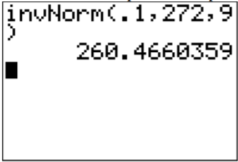
- Find the length of pregnancy that 10% of all pregnancies last less than.
- Suppose you meet a woman who says that she was pregnant for less than 250 days. Would this be unusual and what might you think?
a. x = length of a human pregnancy
b. First translate the statement into a mathematical statement.
P (x>280)
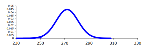
Now, draw a picture. Remember the center of this normal curve is 272.
.png?revision=1 "problem solving with the normal distribution")
To find the probability on the TI-83/84, looking at the picture you realize the lower limit is 280. The upper limit is infinity. The calculator doesn’t have infinity on it, so you need to put in a really big number. Some people like to put in 1000, but if you are working with numbers that are bigger than 1000, then you would have to remember to change the upper limit. The safest number to use is \(1 \times 10^{99}\), which you put in the calculator as 1E99 (where E is the EE button on the calculator). The command looks like:
\(\text{normalcdf}(280,1 E 99,272,9)\)
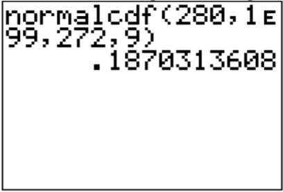.png?revision=1 "problem solving with the normal distribution")
Thus 18.7% of all pregnancies last more than 280 days. This is not unusual since the probability is greater than 5%.
c. First translate the statement into a mathematical statement.
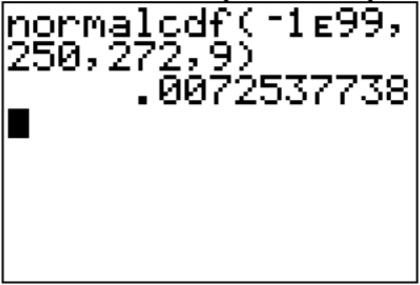
P (x<250)
.png?revision=1 "problem solving with the normal distribution")
To find the probability on the TI-83/84, looking at the picture, though it is hard to see in this case, the lower limit is negative infinity. Again, the calculator doesn’t have this on it, put in a really small number, such as \(-1 \times 10^{99}=-1 E 99\) on the calculator.
.png?revision=1 "problem solving with the normal distribution")
\(P(x<250)=\text { normalcdf }(-1 E 99,250,272,9)=0.0073\)
Thus 0.73% of all pregnancies last less than 250 days. This is unusual since the probability is less than 5%.
d. First translate the statement into a mathematical statement.
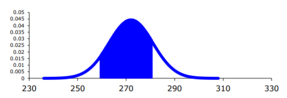
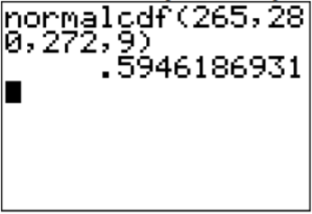
\(P(265<x<280)\)
.png?revision=1 "problem solving with the normal distribution")
In this case, the lower limit is 265 and the upper limit is 280.
Using the calculator
.png?revision=1 "problem solving with the normal distribution")
\(P(265<x<280)=\text { normalcdf }(265,280,272,9)=0.595\)
Many software programs always give you the area to the left. So \(P(x<280)\) is the area to the left of 280 and \(P(x<265)\) is the area to the left of 265. So the area is between the two would be the bigger one minus the smaller one. So, \(P(265<x<280)= P(x<280) - P(x<265) =0.595\). Thus 59.5% of all pregnancies last between 265 and 280 days.
e. This problem is asking you to find an x value from a probability. You want to find the x value that has 10% of the length of pregnancies to the left of it. On the TI-83/84, the command is in the DISTR menu and is called invNorm(. The invNorm( command needs the area to the left. In this case, that is the area you are given. For the command on the calculator, once you have invNorm( on the main screen you type in the probability to the left, mean, standard deviation, in that order with the commas.
.png?revision=1 "problem solving with the normal distribution")
Thus 10% of all pregnancies last less than approximately 260 days.
f. From part (c) you found the probability that a pregnancy lasts less than 250 days is 0.73%. Since this is less than 5%, it is very unusual. You would think that either the woman had a premature baby, or that she may be wrong about when she actually became pregnant.
Example \(\PageIndex{2}\) general normal distribution
The mean mathematics SAT score in 2012 was 514 with a standard deviation of 117 ("Total group profile," 2012). Assume the mathematics SAT score is normally distributed.
- Find the probability that a person has a mathematics SAT score over 700.
- Find the probability that a person has a mathematics SAT score of less than 400.
- Find the probability that a person has a mathematics SAT score between a 500 and a 650.
- Find the mathematics SAT score that represents the top 1% of all scores.
a. x = mathematics SAT score
P (x>700)
Now, draw a picture. Remember the center of this normal curve is 514.
.png?revision=1 "problem solving with the normal distribution")
On TI-83/84: \(P(x>700)=\text { normalcdf }(700,1 E 99,514,117) \approx 0.056\)
On R: \(P(x>700)=1-\text { pnorm }(700,514,117) \approx 0.056\)
There is a 5.6% chance that a person scored above a 700 on the mathematics SAT test. This is not unusual.
P (x<400)
.png?revision=1 "problem solving with the normal distribution")
On TI-83/84: \(P(x<400)=\text { normalcdf }(-1 E 99,400,514,117) \approx 0.165\)
On R: \(P(x<400)=\operatorname{pnorm}(400,514,117) \approx 0.165\)
So, there is a 16.5% chance that a person scores less than a 400 on the mathematics part of the SAT.
P (500<x<650)
.png?revision=1 "problem solving with the normal distribution")
On TI-83/84: \(P(500<x<650)=\text { normalcdf }(500,650,514,117) \approx 0.425\)
On R: \(P(500<x<650)=\text { pnorm }(650,514,117)-\text { pnorm }(500,514,117) \approx 0.425\)
So, there is a 42.5% chance that a person has a mathematical SAT score between 500 and 650.
e. This problem is asking you to find an x value from a probability. You want to find the x value that has 1% of the mathematics SAT scores to the right of it. Remember, the calculator and R always need the area to the left, you need to find the area to the left by 1 - 0.01 = 0.99.
On TI-83/84: \(\text{invNorm}(.99,514,117) \approx 786\)
On R: \(\text{qnorm}(.99,514,117) \approx 786\)
So, 1% of all people who took the SAT scored over about 786 points on the mathematics SAT.
Exercise \(\PageIndex{1}\)
- P (z<2.36)
- P (z>0.67)
- P (0<z<2.11)
- P (-2.78<z<1.97)
- The area to the left of z is 15%.
- The area to the right of z is 65%.
- The area to the left of z is 10%.
- The area to the right of z is 5%.
- The area between -z and z is 95%. (Hint draw a picture and figure out the area to the left of the -z.)
- The area between -z and z is 99%.
- Find the probability that a person in China has blood pressure of 135 mmHg or more.
- Find the probability that a person in China has blood pressure of 141 mmHg or less.
- Find the probability that a person in China has blood pressure between 120 and 125 mmHg.
- Is it unusual for a person in China to have a blood pressure of 135 mmHg? Why or why not?
- What blood pressure do 90% of all people in China have less than?
- Find the probability that an Atlantic cod has a length less than 52 cm.
- Find the probability that an Atlantic cod has a length of more than 74 cm.
- Find the probability that an Atlantic cod has a length between 40.5 and 57.5 cm.
- If you found an Atlantic cod to have a length of more than 74 cm, what could you conclude?
- What length are 15% of all Atlantic cod longer than?
- Find the probability that a woman age 45-59 in Ghana, Nigeria, or Seychelles has a cholesterol level above 6.2 mmol/l (considered a high level).
- Find the probability that a woman age 45-59 in Ghana, Nigeria, or Seychelles has a cholesterol level below 5.2 mmol/l (considered a normal level).
- Find the probability that a woman age 45-59 in Ghana, Nigeria, or Seychelles has a cholesterol level between 5.2 and 6.2 mmol/l (considered borderline high).
- If you found a woman age 45-59 in Ghana, Nigeria, or Seychelles having a cholesterol level above 6.2 mmol/l, what could you conclude?
- What value do 5% of all woman ages 45-59 in Ghana, Nigeria, or Seychelles have a cholesterol level less than?
- Find the probability that a man age 40-49 in the U.S. eats more than 110 g of fat every day.
- Find the probability that a man age 40-49 in the U.S. eats less than 93 g of fat every day.
- Find the probability that a man age 40-49 in the U.S. eats less than 65 g of fat every day.
- If you found a man age 40-49 in the U.S. who says he eats less than 65 g of fat every day, would you believe him? Why or why not?
- What daily fat level do 5% of all men age 40-49 in the U.S. eat more than?
- Find the probability that a dishwasher will last more than 15 years.
- Find the probability that a dishwasher will last less than 6 years.
- Find the probability that a dishwasher will last between 8 and 10 years.
- If you found a dishwasher that lasted less than 6 years, would you think that you have a problem with the manufacturing process? Why or why not?
- A manufacturer of dishwashers only wants to replace free of charge 5% of all dishwashers. How long should the manufacturer make the warranty period?
- Find the probability that a starting nurse will make more than $80,000.
- Find the probability that a starting nurse will make less than $60,000.
- Find the probability that a starting nurse will make between $55,000 and $72,000.
- If a nurse made less than $50,000, would you think the nurse was under paid? Why or why not?
- What salary do 30% of all nurses make more than?
- Find the probability that the yearly rainfall is less than 100 mm.
- Find the probability that the yearly rainfall is more than 240 mm.
- Find the probability that the yearly rainfall is between 140 and 250 mm.
- If a year has a rainfall less than 100mm, does that mean it is an unusually dry year? Why or why not?
- What rainfall amount are 90% of all yearly rainfalls more than?
1. a. \(P(z<2.36)=0.9909\), b. \(P(z>0.67)=0.2514\), c. \(P(0<z<2.11)=0.4826\), d. \(P(-2.78<z<1.97)=0.9729\)
3. a. -0.6667, b. -2.6667, c. -2, d. 6.6667
5. a. See solutions, b. \(P(x<52 \mathrm{cm})=0.7128\), c. \(P(x>74 \mathrm{cm})=5.852 \times 10^{-11}\), d. \(P(40.5 \mathrm{cm}<x<57.5 \mathrm{cm})=0.9729\), e. See solutions, f. 53.8 cm
7. a. See solutions, b. \(P(x>110 \mathrm{g})=0.0551\) c. \(P(x<93 \mathrm{g})=0.0097\), d. \(P(x<65 \mathrm{g}) \approx 0\) or \(5.57 \times 10^{-19}\), e. See solutions, f. 110.2 g
9. a. See solutions, b. \(P(x>\$ 80,000)=0.1168\), c. \(P(x>\$ 80,000)=0.2283\), d. \(P(\$ 55,000<x<\$ 72,000)=0.5519\), e. See solutions, f. $73,112
Normal Distribution
In these lessons, we learn the characteristics of the normal distribution and its applications.
Related Pages Normal Distribution Normal Distribution: Probability Standard Deviation More Lessons for Statistics Math Worksheets
What is the Normal Distribution? Probably the most widely known and used of all distributions is the normal distribution. It fits many human characteristics, such as height, weight, speed etc. Many living things in nature, such as trees, animals and insects have many characteristics that are normally distributed. Many variables in business and industry are also normally distributed.
Discovery of the normal curve is generally credited to Karl Gauss (1777 – 1855), who recognized that the errors of repeated measurement of objects are often normally distributed. Sometimes, the normal distribution is also called the Gaussian distribution.
The normal distribution has the following characteristics:
- It is a continuous distribution
- It is symmetrical about the mean. Each half of the distribution is a mirror image of the other half.
- It is asymptotic to the horizontal axis. That is, it does not touch the x -axis and it goes on forever in each direction.
- It is unimodal. The normal curve is sometimes called a bell-shaped curve. All the values are “bunched up” in only one portion of the graph – the center of the curve.
- It is a family of curves. Every unique value of the mean and every unique value of the standard deviation result in a different normal curve.
- The area under the curve is 1. The area under the curve yields the probabilities, so the total of all probabilities for a normal distribution is 1. Since the distribution is symmetric, the area of the distribution on each side of the mean is 0.5.
What is the Probability density function of the normal distribution? The normal distribution is described by two parameters: the mean, μ, and the standard deviation, σ. We write X - N(μ, σ 2 ).
The following diagram shows the formula for Normal Distribution. Scroll down the page for more examples and solutions on using the normal distribution formula.

Since the formula is so complex, using it to determine area under the curve is cumbersome and time consuming. Instead, tables and software are used to find the probabilities for the normal distribution. This will be discussed in the lesson on Z-Score .
Normal Distribution The 68-95-99.7 Rule
- Approximately 68% of the data falls ±1 standard deviation from the mean.
- Approximately 95% of the data falls ±2 standard deviation from the mean.
- Approximately 99.7% of the data falls ±3 standard deviation from the mean.
In a call center, the distribution of the number of phone calls answered each day by each of the 12 receptionists is bell-shaped and has a mean of 63 and a standard deviation of 3. Use the empirical rule, what is the approximate percentage of daily phone calls numbering between 60 and 66?
The scores of a midterm are normally distributed with a mean of 85% and a standard deviation of 6%. Find the percentage of the class that score above and below the given score. Use the 68-95-99.7 rule from the text. a) Score: 91% b) Score: 73%
The following video explores the normal distribution
Presentation on spreadsheet to show that the normal distribution approximates the binomial distribution for a large number of trials.

We welcome your feedback, comments and questions about this site or page. Please submit your feedback or enquiries via our Feedback page.
How to do Normal Distributions Calculations
This guide will show you how to calculate the probability (area under the curve) of a standard normal distribution. It will first show you how to interpret a Standard Normal Distribution Table. It will then show you how to calculate the:
- probability less than a z-value
- probability greater than a z-value
- probability between z-values
- probability outside two z-values .
We have a calculator that calculates probabilities based on z-values for all the above situations. In addition, it also outputs all the working to get to the answer, so you know the logic of how to calculate the answer.
How to Use the Standard Normal Distribution Table
The most common form of standard normal distribution table that you see is a table similar to the one below (click image to enlarge):

The Standard Normal Distribution Table
The standard normal distribution table provides the probability that a normally distributed random variable Z, with mean equal to 0 and variance equal to 1, is less than or equal to z. It does this for positive values of z only (i.e., z-values on the right-hand side of the mean). What this means in practice is that if someone asks you to find the probability of a value being less than a specific, positive z-value, you can simply look that value up in the table. We call this area Φ. Thus, for this table, P(Z < a) = Φ(a), where a is positive.
Diagrammatically, the probability of Z less than ' a ' being Φ(a), as determined from the standard normal distribution table, is shown below:

Probability less than a z-value
P(Z < –a)
As explained above, the standard normal distribution table only provides the probability for values less than a positive z-value (i.e., z-values on the right-hand side of the mean). So how do we calculate the probability below a negative z-value (as illustrated below)?

We start by remembering that the standard normal distribution has a total area (probability) equal to 1 and it is also symmetrical about the mean. Thus, we can do the following to calculate negative z-values: we need to appreciate that the area under the curve covered by P(Z > a) is the same as the probability less than –a {P(Z < –a)} as illustrated below:

Making this connection is very important because from the standard normal distribution table, we can calculate the probability less than ' a ', as ' a ' is now a positive value. Imposing P(Z < a) on the above graph is illustrated below:

From the above illustration, and from our knowledge that the area under the standard normal distribution is equal to 1, we can conclude that the two areas add up to 1. We can, therefore, make the following statements:
Φ(a) + Φ(–a) = 1 ∴ Φ(–a) = 1 – Φ(a)
Thus, we know that to find a value less than a negative z-value we use the following equation:
Φ(–a) = 1 – Φ(a), e.g. Φ(–1.43) = 1 – Φ(1.43)
Probability greater than a z-value
The probability of P(Z > a) is: 1 – Φ(a). To understand the reasoning behind this look at the illustration below:

You know Φ(a) and you know that the total area under the standard normal curve is 1 so by mathematical deduction: P(Z > a) is: 1 - Φ(a).
P(Z > –a)
The probability of P(Z > –a) is P(a), which is Φ(a). To understand this we need to appreciate the symmetry of the standard normal distribution curve. We are trying to find out the area below:

But by reflecting the area around the centre line (mean) we get the following:

Notice that this is the same size area as the area we are looking for, only we already know this area, as we can get it straight from the standard normal distribution table: it is P(Z < a). Therefore, the P(Z > –a) is P(Z < a), which is Φ (a).
Probability between z-values
You are wanting to solve the following:

The key requirement to solve the probability between z-values is to understand that the probability between z-values is the difference between the probability of the greatest z-value and the lowest z-value:
P(a < Z < b) = P(Z < b) – P(Z < a)
which is illustrated below:

P(a < Z < b)
The probability of P(a < Z < b) is calculated as follows.
First separate the terms as the difference between z-scores:
P(a < Z < b) = P(Z < b) – P( Z < a) (explained in the section above)
Then express these as their respective probabilities under the standard normal distribution curve:
P(Z < b) – P(Z < a) = Φ(b) – Φ(a).
Therefore, P(a < Z < b) = Φ(b) – Φ(a), where a and b are positive.
P(–a < Z < b)
The probability of P(–a < Z < b) is illustrated below:

P(–a < Z < b) = P(Z < b) – P(Z < –a)
P(Z < b) – P(Z < –a) = Φ(b) – Φ(–a) = Φ(b) – {1 – Φ(a)} P(Z < –a) explained above .
∴ P(–a < Z < b) = Φ(b) – {1 – Φ(a)}, where a is negative and b is positive.
P(–a < Z < –b)
The probability of P(–a < Z < –b) is illustrated below:

P(–a < Z < –b) = P(Z < –b) – P( Z < –a)
P(Z < b) – P(Z < –a) = Φ(–b) – Φ(–a) = {1 – Φ(b)} – {1 – Φ(a)} P(Z < –a) explained above . = 1 – Φ(b) – 1 + Φ(a) = Φ(a) – Φ(b)
The above calculations can also be seen clearly in the diagram below:

Notice that the reflection results in a and b "swapping positions".

Probability outside of a range of z-values
An illustration of this type of problem is found below:

To solve these types of problems, you simply need to work out each separate area under the standard normal distribution curve and then add the probabilities together. This will give you the total probability.
When a is negative and b is positive (as above) the total probability is:
P(Z < –a) + P(Z > b) = Φ(–a) + {1 – Φ(b)} P(Z > b) explained above . = {1 – Φ(a)} + {1 – Φ(b)} P(Z < –a) explained above . = 1 – Φ(a) + 1 – Φ(b) = 2 – Φ(a) – Φ(b)
When a and b are negative as illustrated below:

The total probability is:
P(Z < –a) + P(Z > –b) = Φ(–a) + Φ(b) P(Z > –b) explained above . = {1 – Φ(a)} + Φ(b) P(Z < –a) explained above . = 1 + Φ(b) – Φ(a)
When a and b are positive as illustrated below:

P(Z < a) + P(Z > b) = Φ(a) + {1 – Φ(b)} P(Z > b) explained above . = 1 + Φ(a) – Φ(b)
Check out our calculator to get some practice in!
Have a language expert improve your writing
Run a free plagiarism check in 10 minutes, generate accurate citations for free.
- Knowledge Base
- Normal Distribution | Examples, Formulas, & Uses
Normal Distribution | Examples, Formulas, & Uses
Published on October 23, 2020 by Pritha Bhandari . Revised on June 21, 2023.
In a normal distribution, data is symmetrically distributed with no skew . When plotted on a graph, the data follows a bell shape, with most values clustering around a central region and tapering off as they go further away from the center.
Normal distributions are also called Gaussian distributions or bell curves because of their shape.

Table of contents
Why do normal distributions matter, what are the properties of normal distributions, empirical rule, central limit theorem, formula of the normal curve, what is the standard normal distribution, other interesting articles, frequently asked questions about normal distributions.
All kinds of variables in natural and social sciences are normally or approximately normally distributed. Height, birth weight, reading ability, job satisfaction, or SAT scores are just a few examples of such variables.
Because normally distributed variables are so common, many statistical tests are designed for normally distributed populations.
Understanding the properties of normal distributions means you can use inferential statistics to compare different groups and make estimates about populations using samples.
Prevent plagiarism. Run a free check.
Normal distributions have key characteristics that are easy to spot in graphs:
- The mean , median and mode are exactly the same.
- The distribution is symmetric about the mean—half the values fall below the mean and half above the mean.
- The distribution can be described by two values: the mean and the standard deviation .

The mean is the location parameter while the standard deviation is the scale parameter.
The mean determines where the peak of the curve is centered. Increasing the mean moves the curve right, while decreasing it moves the curve left.

The standard deviation stretches or squeezes the curve. A small standard deviation results in a narrow curve, while a large standard deviation leads to a wide curve.

The empirical rule , or the 68-95-99.7 rule, tells you where most of your values lie in a normal distribution:
- Around 68% of values are within 1 standard deviation from the mean.
- Around 95% of values are within 2 standard deviations from the mean.
- Around 99.7% of values are within 3 standard deviations from the mean.
Following the empirical rule:
- Around 68% of scores are between 1,000 and 1,300, 1 standard deviation above and below the mean.
- Around 95% of scores are between 850 and 1,450, 2 standard deviations above and below the mean.
- Around 99.7% of scores are between 700 and 1,600, 3 standard deviations above and below the mean.

The empirical rule is a quick way to get an overview of your data and check for any outliers or extreme values that don’t follow this pattern.
If data from small samples do not closely follow this pattern, then other distributions like the t-distribution may be more appropriate. Once you identify the distribution of your variable, you can apply appropriate statistical tests.
The central limit theorem is the basis for how normal distributions work in statistics.
In research, to get a good idea of a population mean, ideally you’d collect data from multiple random samples within the population. A sampling distribution of the mean is the distribution of the means of these different samples.
The central limit theorem shows the following:
- Law of Large Numbers: As you increase sample size (or the number of samples), then the sample mean will approach the population mean.
- With multiple large samples, the sampling distribution of the mean is normally distributed, even if your original variable is not normally distributed.
Parametric statistical tests typically assume that samples come from normally distributed populations, but the central limit theorem means that this assumption isn’t necessary to meet when you have a large enough sample.
You can use parametric tests for large samples from populations with any kind of distribution as long as other important assumptions are met. A sample size of 30 or more is generally considered large.
For small samples, the assumption of normality is important because the sampling distribution of the mean isn’t known. For accurate results, you have to be sure that the population is normally distributed before you can use parametric tests with small samples.
Once you have the mean and standard deviation of a normal distribution, you can fit a normal curve to your data using a probability density function .

In a probability density function, the area under the curve tells you probability. The normal distribution is a probability distribution , so the total area under the curve is always 1 or 100%.
The formula for the normal probability density function looks fairly complicated. But to use it, you only need to know the population mean and standard deviation.
For any value of x , you can plug in the mean and standard deviation into the formula to find the probability density of the variable taking on that value of x .
On your graph of the probability density function, the probability is the shaded area under the curve that lies to the right of where your SAT scores equal 1380.

The standard normal distribution , also called the z -distribution , is a special normal distribution where the mean is 0 and the standard deviation is 1.
Every normal distribution is a version of the standard normal distribution that’s been stretched or squeezed and moved horizontally right or left.

While individual observations from normal distributions are referred to as x , they are referred to as z in the z -distribution. Every normal distribution can be converted to the standard normal distribution by turning the individual values into z -scores.
Z -scores tell you how many standard deviations away from the mean each value lies.

You only need to know the mean and standard deviation of your distribution to find the z -score of a value.
We convert normal distributions into the standard normal distribution for several reasons:
- To find the probability of observations in a distribution falling above or below a given value.
- To find the probability that a sample mean significantly differs from a known population mean.
- To compare scores on different distributions with different means and standard deviations.
Finding probability using the z -distribution
Each z -score is associated with a probability, or p -value , that tells you the likelihood of values below that z -score occurring. If you convert an individual value into a z -score, you can then find the probability of all values up to that value occurring in a normal distribution.
The mean of our distribution is 1150, and the standard deviation is 150. The z -score tells you how many standard deviations away 1380 is from the mean.
For a z -score of 1.53, the p -value is 0.937. This is the probability of SAT scores being 1380 or less (93.7%), and it’s the area under the curve left of the shaded area.

To find the shaded area, you take away 0.937 from 1, which is the total area under the curve.
Probability of x > 1380 = 1 – 0.937 = 0.063
If you want to know more about statistics , methodology , or research bias , make sure to check out some of our other articles with explanations and examples.
- Student’s t table
- Student’s t distribution
- Descriptive statistics
- Measures of central tendency
- Correlation coefficient
Methodology
- Cluster sampling
- Stratified sampling
- Types of interviews
- Cohort study
- Thematic analysis
Research bias
- Implicit bias
- Cognitive bias
- Survivorship bias
- Availability heuristic
- Nonresponse bias
- Regression to the mean
In a normal distribution , data are symmetrically distributed with no skew. Most values cluster around a central region, with values tapering off as they go further away from the center.
The measures of central tendency (mean, mode, and median) are exactly the same in a normal distribution.

The standard normal distribution , also called the z -distribution, is a special normal distribution where the mean is 0 and the standard deviation is 1.
Any normal distribution can be converted into the standard normal distribution by turning the individual values into z -scores. In a z -distribution, z -scores tell you how many standard deviations away from the mean each value lies.
The empirical rule, or the 68-95-99.7 rule, tells you where most of the values lie in a normal distribution :
- Around 68% of values are within 1 standard deviation of the mean.
- Around 95% of values are within 2 standard deviations of the mean.
- Around 99.7% of values are within 3 standard deviations of the mean.
The t -distribution is a way of describing a set of observations where most observations fall close to the mean , and the rest of the observations make up the tails on either side. It is a type of normal distribution used for smaller sample sizes, where the variance in the data is unknown.
The t -distribution forms a bell curve when plotted on a graph. It can be described mathematically using the mean and the standard deviation .
Cite this Scribbr article
If you want to cite this source, you can copy and paste the citation or click the “Cite this Scribbr article” button to automatically add the citation to our free Citation Generator.
Bhandari, P. (2023, June 21). Normal Distribution | Examples, Formulas, & Uses. Scribbr. Retrieved April 1, 2024, from https://www.scribbr.com/statistics/normal-distribution/
Is this article helpful?

Pritha Bhandari
Other students also liked, t-distribution: what it is and how to use it, the standard normal distribution | calculator, examples & uses, understanding p values | definition and examples, what is your plagiarism score.

- school Campus Bookshelves
- menu_book Bookshelves
- perm_media Learning Objects
- login Login
- how_to_reg Request Instructor Account
- hub Instructor Commons
- Download Page (PDF)
- Download Full Book (PDF)
- Periodic Table
- Physics Constants
- Scientific Calculator
- Reference & Cite
- Tools expand_more
- Readability
selected template will load here
This action is not available.
11.3: Application of Normal Distributions
- Last updated
- Save as PDF
- Page ID 59991

- Darlene Diaz
- Santiago Canyon College via ASCCC Open Educational Resources Initiative
Learning Objectives
- Apply the characteristics of a normal distribution to solving applications.
Introduction
The normal distribution is the foundation for statistical inference and will be an essential part of many of those topics in later chapters. In the meantime, this section will cover some of the types of questions that can be answered using the properties of a normal distribution. The first examples deal with more theoretical questions that will help you master basic understandings and computational skills, while the later problems will provide examples with real data, or at least a real context.
Normal Distributions with Real Data
The foundation of performing experiments by collecting surveys and samples is most often based on the normal distribution, as you will learn in greater detail in later chapters. Here are two examples to get you started.
Example \(\PageIndex{1}\)
The Information Centre of the National Health Service in Britain collects and publishes a great deal of information and statistics on health issues affecting the population. One such comprehensive data set tracks information about the health of children [1]. According to its statistics, in 2006, the mean height of 12-year-old boys was 152.9 cm, with a standard deviation estimate of approximately 8.5 cm. (These are not the exact figures for the population, and in later chapters, we will learn how they are calculated and how accurate they may be, but for now, we will assume that they are a reasonable estimate of the true parameters.) If 12-year-old Cecil is 158 cm, approximately what percentage of all 12-year-old boys in Britain is he taller than?
We first must assume that the height of 12-year-old boys in Britain is normally distributed, and this seems like a reasonable assumption to make. As always, draw a sketch and estimate a reasonable answer prior to calculating the percentage. In this case, let’s use the calculator to sketch the distribution and the shading. First, decide on an appropriate window that includes about 3 standard deviations on either side of the mean. In this case, 3 standard deviations is about 25.5 cm, so add and subtract this value to/from the mean to find the horizontal extremes. Then enter the appropriate ‘ShadeNorm(’ command as shown:

From this data, we would estimate that Cecil is taller than about 73% of 12-year-old boys. We could also phrase our assumption this way: the probability of a randomly selected British 12- year-old boy being shorter than Cecil is about 0.73. Often with data like this, we use percentiles. We would say that Cecil is in the 73 rd percentile for height among 12-year-old boys in Britain.
How tall would Cecil need to be in order to be in the top 1% of all 12-year-old boys in Britain?
Here is a sketch:

In this case, we are given the percentage, so we need to use the ‘invNorm(’ command as shown.

Our results indicate that Cecil would need to be about 173 cm tall to be in the top 1% of 12-year-old boys in Britain.
Example \(\PageIndex{2}\)
Suppose that the distribution of the masses of female marine iguanas in Puerto Villamil in the Galapagos Islands is approximately normal, with a mean mass of 950 g and a standard deviation of 325 g. There are very few young marine iguanas in the populated areas of the islands, because feral cats tend to kill them. How rare is it that we would find a female marine iguana with a mass less than 400 g in this area?

Using a graphing calculator, we can approximate the probability of a female marine iguana being less than 400 grams as follows:

With a probability of approximately 0.045, or only about 5%, we could say it is rather unlikely that we would find an iguana this small.
Example \(\PageIndex{3}\)
The physical plant at the main campus of a large state university receives daily requests to replace florescent lightbulbs. The distribution of the number of daily requests is bell-shaped and has a mean of 59 and a standard deviation of 9. Using the Empirical rule, what is the approximate percentage of lightbulb replacement requests numbering between 59 and 77?
Since we want to use the Empirical Rule, we should draw a figure reflecting the Empirical Rule given the mean is \(59\) and the standard deviation is \(9\). Recall, 1 standard deviation from the mean is \(59 ± 9\), two standard deviations from the mean is \(59 ± 2 \cdot 9\), and 3 standard deviations from the mean is \(59 ± 3 \cdot 9\).

Once we make this figure, we can easily the percentage of lightbulb replacement requests numbering between 59 and 77:
\(34 \% + 13.5 \% = 47.5 \%\)
Thus, \(47.5 \%\) of lightbulb replacement requests numbering between 59 and 77.
Example \(\PageIndex{4}\)
A company has a policy of retiring company cars; this policy looks at number of miles driven, purpose of trips, style of car and other features. The distribution of the number of months in service for the fleet of cars is bell-shaped and has a mean of 41 months and a standard deviation of 5 months. Using the Empirical Rule, what is the approximate percentage of cars that remain in service between 46 and 56 months?
Since we want to use the Empirical Rule, we should draw a figure reflecting the Empirical Rule given the mean is 41 and the standard deviation is 5:

Once we make this figure, we can easily the approximate percentage of cars that remain in service between 46 and 56 months:
\(13.5 \% + 2.35 \% = 15.85 \%\)
Thus, \(15.85 \%\) of cars remain in service between 46 and 56 months.
1. Which of the following intervals contains the middle 95% of the data in a standard normal distribution?
a) \(z < 2\)
b) \(z ≤ 1.645\)
c) \(z ≤ 1.96\)
d) \(−1.645 ≤ z ≤ 1.645\)
e) \(−1.96 ≤ z ≤ 1.96\)
2. The manufacturing process at a metal-parts factory produces some slight variation in the diameter of metal ball bearings. The quality control experts claim that the bearings produced have a mean diameter of 1.4 cm. If the diameter is more than 0.0035 cm too wide or too narrow, they will not work properly. In order to maintain its reliable reputation, the company wishes to ensure that no more than one-tenth of 1% of the bearings that are made are ineffective. What would the standard deviation of the manufactured bearings need to be in order to meet this goal?
3. Suppose that the wrapper of a certain candy bar lists its weight as 2.13 ounces. Naturally, the weights of individual bars vary somewhat. Suppose that the weights of these candy bars vary according to a normal distribution, with \(µ = 2.2\) ounces and \(σ = 0.04\) ounces.
a) What proportion of the candy bars weigh less than the advertised weight?
b) What proportion of the candy bars weight between 2.2 and 2.3 ounces?
c) A candy bar of what weight would be heavier than all but 1% of the candy bars out there?
d) If the manufacturer wants to adjust the production process so that no more than 1 candy bar in 1000 weighs less than the advertised weight, what would the mean of the actual weights need to be? (Assume the standard deviation remains the same.)
e) If the manufacturer wants to adjust the production process so that the mean remains at 2.2 ounces and no more than 1 candy bar in 1000 weighs less than the advertised weight, how small does the standard deviation of the weights need to be?
4. The Acme Company manufactures widgets. The distribution of widget weights is bell-shaped. The widget weights have a mean of 51 ounces and a standard deviation of 4 ounces. Use the Empirical Rule to answer the following questions.
a) 99.7% of the widget weights lie between what two weights?
b) What percentage of the widget weights lie between 43 and 63 ounces?
c) What percentage of the widget weights lie above 47?
BUS204: Business Statistics
Practice: The Normal Distribution
Solve these problems, then check your answers against the given solutions.
According to a study done by De Anza students, the height for Asian adult males is normally distributed with an average of 66 inches and a standard deviation of 2.5 inches. Suppose one Asian adult male is randomly chosen. Let X =height of the individual.
- X ~____ ( ____, ____)
- Find the probability that the person is between 65 and 69 inches. Include a sketch of the graph and write a probability statement.
- Would you expect to meet many Asian adult males over 72 inches? Explain why or why not, and justify your answer numerically.
- The middle 40% of heights fall between what two values? Sketch the graph and write the probability statement.
The percent of fat calories that a person in America consumes each day is normally distributed with a mean of about 36 and a standard deviation of 10. Suppose that one individual is randomly chosen. Let X =percent of fat calories.
- X ~_____ (_____, _____ )
- Find the probability that the percent of fat calories a person consumes is more than 40. Graph the situation. Shade in the area to be determined.
- Find the maximum number for the lower quarter of percent of fat calories. Sketch the graph and write the probability statement.
Suppose that the distance of fly balls hit to the outfield (in baseball) is normally distributed with a mean of 250 feet and a standard deviation of 50 feet.
- If X = distance in feet for a fly ball, then X~____ (____ ,____ )
- If one fly ball is randomly chosen from this distribution, what is the probability that this ball traveled fewer than 220 feet? Sketch the graph. Scale the horizontal axis X. Shade the region corresponding to the probability. Find the probability.
- Find the 80th percentile of the distribution of fly balls. Sketch the graph and write the probability statement.
In China, 4-year-olds average 3 hours a day unsupervised. Most of the unsupervised children live in rural areas, considered safe. Suppose that the standard deviation is 1.5 hours and the amount of time spent alone is normally distributed. We randomly survey one Chinese 4-year-old living in a rural area. We are interested in the amount of time the child spends alone per day.
- In words, define the random variable X. X =
- Find the probability that the child spends less than 1 hour per day unsupervised. Sketch the graph and write the probability statement.
- What percent of the children spend over 10 hours per day unsupervised?
- 70% of the children spend at least how long per day unsupervised?
In the 1992 presidential election, Alaska's 40 election districts averaged 1956.8 votes per district for President Clinton. The standard deviation was 572.3. (There are only 40 election districts in Alaska.) The distribution of the votes per district for President Clinton was bell-shaped. Let X = number of votes for President Clinton for an election district.
- State the approximate distribution of X. X~
- Is 1956.8 a population mean or a sample mean? How do you know?
- Find the probability that a randomly selected district had fewer than 1600 votes for President Clinton. Sketch the graph and write the probability statement.
- Find the probability that a randomly selected district had between 1800 and 2000 votes for President Clinton.
- Find the third quartile for votes for President Clinton.
Suppose that the duration of a particular type of criminal trial is known to be normally distributed with a mean of 21 days and a standard deviation of 7 days.
- If one of the trials is randomly chosen, find the probability that it lasted at least 24 days. Sketch the graph and write the probability statement.
- 60% of all of these types of trials are completed within how many days?
Terri Vogel, an amateur motorcycle racer, averages 129.71 seconds per 2.5 mile lap (in a 7 lap race) with a standard deviation of 2.28 seconds . The distribution of her race times is normally distributed. We are interested in one of her randomly selected laps.
- Find the percent of her laps that are completed in less than 130 seconds.
- The fastest 3% of her laps are under .
- The middle 80% of her laps are from seconds to seconds.
Thuy Dau, Ngoc Bui, Sam Su, and Lan Voung conducted a survey as to how long customers at Lucky claimed to wait in the checkout line until their turn. Let X =time in line. Below are the ordered real data (in minutes):
- Calculate the sample mean and the sample standard deviation.
- Construct a histogram. Start the x — axis at —0.375 and make bar widths of 2 minutes.
- Draw a smooth curve through the midpoints of the tops of the bars.
- In words, describe the shape of your histogram and smooth curve.
- e. Let the sample mean approximate μ and the sample standard deviation approximate σ. The distribution of X can then be approximated by X ~
- Use the distribution in (e) to calculate the probability that a person will wait fewer than 6.1 minutes.
- Determine the cumulative relative frequency for waiting less than 6.1 minutes.
- Why aren't the answers to (f) and (g) exactly the same?
- Why are the answers to (f) and (g) as close as they are?
- If only 10 customers were surveyed instead of 50, do you think the answers to (f) and (g) would have been closer together or farther apart? Explain your conclusion.
Suppose that Ricardo and Anita attend different colleges. Ricardo's GPA is the same as the average GPA at his school. Anita's GPA is 0.70 standard deviations above her school average. In complete sentences, explain why each of the following statements may be false.
- Ricardo's actual GPA is lower than Anita's actual GPA.
- Ricardo is not passing since his z-score is zero.
- Anita is in the 70th percentile of students at her college.
Exercise 10
Below is a sample of the maximum capacity (maximum number of spectators) of sports stadiums. The table does not include horse racing or motor racing stadiums.
- Calculate the sample mean and the sample standard deviation for the maximum capacity of sports stadiums (the data).
- Construct a histogram of the data.
- Draw a smooth curve through the midpoints of the tops of the bars of the histogram.
- Let the sample mean approximate μ and the sample standard deviation approximate σ. The distribution of X can then be approximated by X~
- Use the distribution in (e) to calculate the probability that the maximum capacity of sports stadiums is less than 67,000 spectators.
- Determine the cumulative relative frequency that the maximum capacity of sports stadiums is less than 67,000 spectators. Hint: Order the data and count the sports stadiums that have a maximum capacity less than 67,000. Divide by the total number of sports stadiums in the sample.
Try These Multiple Choice Questions
The questions below refer to the following: The patient recovery time from a particular surgical proce- dure is normally distributed with a mean of 5.3 days and a standard deviation of 2.1 days.
Exercise 11
What is the median recovery time?
Exercise 12
What is the z-score for a patient who takes 10 days to recover?
Exercise 13
What is the probability of spending more than 2 days in recovery?
Exercise 14
The 90th percentile for recovery times is?
The questions below refer to the following : The length of time to find a parking space at 9 A.M. follows a normal distribution with a mean of 5 minutes and a standard deviation of 2 minutes.
Exercise 15
Based upon the above information and numerically justified, would you be surprised if it took less than 1 minute to find a parking space?
- Unable to determine
Exercise 16
Find the probability that it takes at least 8 minutes to find a parking space.
Exercise 17
Seventy percent of the time, it takes more than how many minutes to find a parking space?
Exercise 18
If the mean is significantly greater than the standard deviation, which of the following statements is true?
- The data cannot follow the uniform distribution.
- The data cannot follow the exponential distribution..
- The data cannot follow the normal distribution.
- I, II, and III

If you're seeing this message, it means we're having trouble loading external resources on our website.
If you're behind a web filter, please make sure that the domains *.kastatic.org and *.kasandbox.org are unblocked.
To log in and use all the features of Khan Academy, please enable JavaScript in your browser.
AP®︎/College Statistics
Course: ap®︎/college statistics > unit 4.
- Qualitative sense of normal distributions
Normal distribution problems: Empirical rule
- Empirical rule
- Basic normal calculations
Want to join the conversation?
- Upvote Button navigates to signup page
- Downvote Button navigates to signup page
- Flag Button navigates to signup page

Video transcript
IMAGES
VIDEO
COMMENTS
Problems with Solutions. X is a normally distributed variable with mean μ = 30 and standard deviation σ = 4. Find the probabilities. a) P (X < 40) b) P (X > 21) c) P (30 < X < 35) A radar unit is used to measure the speeds of cars on a motorway. The speeds are normally distributed with a mean of 90 km/hr and a standard deviation of 10 km/hr.
Solving Problems Involving Using Normal Distribution . Problem 1: Suppose that the data concerning the first-year salaries of Baruch graduates is normally distributed with the population mean µ = $60000 and the population standard deviation σ = $15000. Find the probability of a randomly selected Baruch graduate earning less than $45000 annually.
Solution: Step 1: Sketch a normal distribution with a mean of μ = 150 cm and a standard deviation of σ = 30 cm . Step 2: The diameter of 120 cm is one standard deviation below the mean. Shade below that point. Step 3: Add the percentages in the shaded area: 0.15 % + 2.35 % + 13.5 % = 16 %.
The distribution is normal with a mean of 25 25, and a standard deviation of 4 4. Everyone who scores in the top 30% 30 % of the distribution gets a certificate. What is the lowest score someone can get and still earn a certificate? The top 5% 5 % of the scores get to compete in a statewide history contest. What is the lowest score someone can ...
Multiply the sample size (found in step 1) by the z-value you found in step 4. For example, 0.300 * 100 = 30. That's it! 2. "More Than" or "Above". This how-to covers solving normal distribution problems that contain the phrase " more than " (or a phrase like "above"). Step 1:Break up the word problem into parts.
This calculus video tutorial provides a basic introduction into normal distribution and probability. It explains how to solve normal distribution problems u...
For normalization purposes. The integral of the rest of the function is square root of 2xpi. So it must be normalized (integral of negative to positive infinity must be equal to 1 in order to define a probability density distribution). Actually, the normal distribution is based on the function exp (-x²/2). If you try to graph that, you'll see ...
Example 16-1. Let \ (X\) denote the IQ (as determined by the Stanford-Binet Intelligence Quotient Test) of a randomly selected American. It has long been known that \ (X\) follows a normal distribution with mean 100 and standard deviation of 16. That is, \ (X\sim N (100, 16^2)\).
Definition 6.3.1 6.3. 1: z-score. z = x − μ σ (6.3.1) (6.3.1) z = x − μ σ. where μ μ = mean of the population of the x value and σ σ = standard deviation for the population of the x value. The z-score is normally distributed, with a mean of 0 and a standard deviation of 1. It is known as the standard normal curve.
Describe the characteristics of the normal distribution. Apply the 68-95-99.7 percent groups to normal distribution datasets. ... There are more problems we can solve using the 68-95-99.7 Rule. but first we must understand what the rule implies. Remember, the rule says that 68% of the data falls within one standard deviation of the mean. ...
The scores of a midterm are normally distributed with a mean of 85% and a standard deviation of 6%. Find the percentage of the class that score above and below the given score. Use the 68-95-99.7 rule from the text. a) Score: 91%. b) Score: 73%. Show Video Lesson. The following video explores the normal distribution.
Introduction. This section will cover some of the types of questions that can be answered using the properties of a normal distribution. The first examples deal with more theoretical questions that will help you master basic understandings and computational skills, while the later problems will provide examples with real data, or at least a real context.
The Standard Normal Distribution Table. The standard normal distribution table provides the probability that a normally distributed random variable Z, with mean equal to 0 and variance equal to 1, is less than or equal to z. It does this for positive values of z only (i.e., z-values on the right-hand side of the mean).
What is a normal distribution and how to use it in statistics? Learn the definition, formulas, examples, and applications of this common data pattern. Find out how to calculate the mean, standard deviation, and z-scores of a normal distribution, and how to compare it with other distributions. Scribbr offers clear and concise explanations, diagrams, and calculators to help you master this topic.
To create a normal distribution, we will draw an idealized curve using something called a density function. The command is called 'normalpdf (', and it is found by pressing [2nd] [DISTR] [1]. Enter an X to represent the random variable, followed by the mean and the standard deviation, all separated by commas.
Apply the characteristics of a normal distribution to solving applications. Introduction. The normal distribution is the foundation for statistical inference and will be an essential part of many of those topics in later chapters. In the meantime, this section will cover some of the types of questions that can be answered using the properties ...
Learn how to solve any Normal Probability Distribution problem. This tutorial first explains the concept behind the normal distribution, then it discusses h...
Solve these problems, then check your answers against the given solutions. Exercises. ... The questions below refer to the following: The length of time to find a parking space at 9 A.M. follows a normal distribution with a mean of 5 minutes and a standard deviation of 2 minutes.
Normal distribution problems: Empirical rule. The empirical rule (also called the "68-95-99.7 rule") is a guideline for how data is distributed in a normal distribution. The rule states that (approximately): - 68% of the data points will fall within one standard deviation of the mean. - 95% of the data points will fall within two standard ...
Normal distribution The normal distribution is the most widely known and used of all distributions. Because the ... That is, rather than directly solve a problem involving a normally distributed variable X with mean µ and standard deviation σ, an indirect approach is used. 1. We first convert the problem into an equivalent one dealing with a ...
This is a great review of the Normal Distribution curve. This video assumes you know the basics. In this video I provide a few problems with the solutions...
Step-by-step solution in solving problems involving normal distribution/curve.
This lecture video covers the concept of solving problems with the normal distribution.Facilitated by Professor Armstrong