All Subjects

Theoretical Statistics
Study guides for every class, that actually explain what's on your next test, multivariate hypothesis testing, from class:.
Multivariate hypothesis testing is a statistical method used to determine whether there are significant differences between multiple groups across several variables simultaneously. This approach extends traditional hypothesis testing to situations where multiple dependent variables are analyzed together, allowing for a more comprehensive understanding of data relationships and group effects. It is particularly useful in contexts where variables may be correlated, thereby capturing the joint behavior of the responses rather than treating them independently.
congrats on reading the definition of Multivariate Hypothesis Testing . now let's actually learn it.
5 Must Know Facts For Your Next Test
- In multivariate hypothesis testing, multiple dependent variables are analyzed simultaneously, enabling the detection of interactions between these variables.
- The multivariate normal distribution plays a crucial role in many multivariate hypothesis tests, as many of these tests assume that the data follows this distribution.
- MANOVA is a common technique used for multivariate hypothesis testing, specifically designed to test hypotheses about group means across multiple dependent variables.
- The rejection region for multivariate tests often involves the use of the Wilks' Lambda statistic, which helps determine if there are significant effects when considering all variables together.
- Assumptions such as multivariate normality and homogeneity of variance-covariance matrices are essential for valid results in multivariate hypothesis testing.
Review Questions
- Multivariate hypothesis testing differs from univariate hypothesis testing by examining multiple dependent variables at once instead of just one. This allows researchers to detect complex interactions and relationships among variables that may not be apparent when looking at them separately. By considering the joint behavior of responses, multivariate methods provide a more comprehensive analysis, capturing correlations and dependencies between the variables.
- Key assumptions necessary for conducting multivariate hypothesis tests include multivariate normality, homogeneity of variance-covariance matrices, and independence of observations. These assumptions are crucial because violating them can lead to inaccurate results and conclusions. For instance, if the data does not follow a multivariate normal distribution, the test statistics may not have their expected distributions, compromising the validity of hypothesis tests like MANOVA.
- Using MANOVA in multivariate hypothesis testing allows for a more holistic approach by assessing differences across all dependent variables simultaneously, which can control for Type I error rates that might inflate when conducting separate ANOVAs. When performing multiple individual ANOVAs, the risk of incorrectly rejecting null hypotheses increases due to multiple comparisons. MANOVA mitigates this risk by providing an overall test statistic and incorporating correlations among dependent variables, offering a clearer picture of group differences in complex datasets.
Related terms
A probability distribution that generalizes the one-dimensional normal distribution to higher dimensions, characterized by a mean vector and a covariance matrix that describes the relationship between multiple variables.
MANOVA : Multivariate Analysis of Variance, a statistical test that assesses whether there are any differences in the mean vectors of multiple groups across two or more dependent variables.
A matrix that provides a measure of the joint variability of multiple random variables, showing how much the variables change together and allowing for the analysis of their relationships.
" Multivariate Hypothesis Testing " also found in:
© 2024 fiveable inc. all rights reserved., ap® and sat® are trademarks registered by the college board, which is not affiliated with, and does not endorse this website..
- > Machine Learning
What is Multivariate Data Analysis?
- Bhumika Dutta
- Aug 23, 2021

Introduction
We have access to huge amounts of data in today’s world and it is very important to analyze and manage the data in order to use it for something important. The words data and analysis go hand in hand, as they depend on each other.
Data analysis and research are also related as they both involve several tools and techniques that are used to predict the outcome of specific tasks for the benefit of any company. The majority of business issues include several factors.
When making choices, managers use a variety of performance indicators and associated metrics. When selecting which items or services to buy, consumers consider a variety of factors. The equities that a broker suggests are influenced by a variety of variables.
When choosing a restaurant, diners evaluate a variety of things. More elements affect managers' and customers' decisions as the world grows more complicated. As a result, business researchers, managers, and consumers must increasingly rely on more sophisticated techniques for data analysis and comprehension.
One of those analytical techniques that are used to read huge amounts of data is known as Multivariate Data Analysis.
(Also read: Binary and multiclass classification in ML )
In statistics, one might have heard of variates, which is a particular combination of different variables. Two of the common variate analysis approaches are univariate and bivariate approaches.
A single variable is statistically tested in univariate analysis, whereas two variables are statistically tested in bivariate analysis. When three or more variables are involved, the problem is intrinsically multidimensional, necessitating the use of multivariate data analysis. In this article, we are going to discuss:
What is multivariate data analysis? Objectives of MVA.
Types of multivariate data analysis.
Advantages of multivariate data analysis.
Disadvantages of multivariate data analysis.
(Recommended read: What is Hypothesis Testing? Types and Methods )
Multivariate data analysis
Multivariate data analysis is a type of statistical analysis that involves more than two dependent variables, resulting in a single outcome. Many problems in the world can be practical examples of multivariate equations as whatever happens in the world happens due to multiple reasons.
One such example of the real world is the weather. The weather at any particular place does not solely depend on the ongoing season, instead many other factors play their specific roles, like humidity, pollution, etc. Just like this, the variables in the analysis are prototypes of real-time situations, products, services, or decision-making involving more variables.
Wishart presented the first article on multivariate data analysis (MVA) in 1928. The topic of the study was the covariance matrix distribution of a normal population with numerous variables.
Hotelling, R. A. Fischer, and others published theoretical work on MVA in the 1930s. multivariate data analysis was widely used in the disciplines of education, psychology, and biology at the time.
As time advanced, MVA was extended to the fields of meteorology, geology, science, and medicine in the mid-1950s. Today, it focuses on two types of statistics: descriptive statistics and inferential statistics. We frequently find the best linear combination of variables that are mathematically docile in the descriptive region, but an inference is an informed estimate that is meant to save analysts time from diving too deeply into the data.
Till now we have talked about the definition and history of multivariate data analysis. Let us learn about the objectives as well.
Objectives of multivariate data analysis:
Multivariate data analysis helps in the reduction and simplification of data as much as possible without losing any important details.
As MVA has multiple variables, the variables are grouped and sorted on the basis of their unique features.
The variables in multivariate data analysis could be dependent or independent. It is important to verify the collected data and analyze the state of the variables.
In multivariate data analysis, it is very important to understand the relationship between all the variables and predict the behavior of the variables based on observations.
It is tested to create a statistical hypothesis based on the parameters of multivariate data. This testing is carried out to determine whether or not the assumptions are true.
(Must read: Hypothesis testing )
Advantages of multivariate data analysis:
The following are the advantages of multivariate data analysis:
As multivariate data analysis deals with multiple variables, all the variables can either be independent or dependent on each other. This helps the analysis to search for factors that can help in drawing accurate conclusions.
Since the analysis is tested, the drawn conclusions are closer to real-life situations.
Disadvantages of multivariate data analysis:
The following are the disadvantages of multivariate data analysis:
Multivariate data analysis includes many complex computations and hence can be laborious.
The analysis necessitates the collection and tabulation of a large number of observations for various variables. This process of observation takes a long time.
(Also read: 15 Statistical Terms for Machine Learning )
7 Types of Multivariate Data Analysis
According to this source , the following types of multivariate data analysis are there in research analysis:
Structural Equation Modelling:
SEM or Structural Equation Modelling is a type of statistical multivariate data analysis technique that analyzes the structural relationships between variables. This is a versatile and extensive data analysis network.
SEM evaluates the dependent and independent variables. In addition, latent variable metrics and model measurement verification are obtained. SEM is a hybrid of metric analysis and structural modeling.
For multivariate data analysis, this takes into account measurement errors and factors observed. The factors are evaluated using multivariate analytic techniques. This is an important component of the SEM model.
(Look also: Statistical data analysis )
Interdependence technique:
The relationships between the variables are studied in this approach to have a better understanding of them. This aids in determining the data's pattern and the variables' assumptions.
Canonical Correlation Analysis:
The canonical correlation analysis deals with the relations of straight lines between two types of variables. It has two main purposes- reduction of data and interpretation of data. Between the two categories of variables, all probability correlations are calculated.
When the two types of correlations are large, interpreting them might be difficult, but canonical correlation analysis can assist to highlight the link between the two variables.
Factor Analysis:
Factor analysis reduces data from a large number of variables to a small number of variables. Dimension reduction is another name for it. Before proceeding with the analysis, this approach is utilized to decrease the data. The patterns are apparent and much easier to examine when factor analysis is completed.
Cluster Analysis:
Cluster analysis is a collection of approaches for categorizing instances or objects into groupings called clusters. The data is divided based on similarity and then labeled to the group throughout the analysis. This is a data mining function that allows them to acquire insight into the data distribution based on each group's distinct characteristics.
Correspondence Analysis:
A table with a two-way array of non-negative values is used in a correspondence analysis approach. This array represents the relationship between the table's row and column entries. A table of contingency, in which the column and row entries relate to the two variables and the numbers in the table cells refer to frequencies, is a popular multivariate data analysis example.
Multidimensional Scaling:
MDS, or multidimensional scaling, is a technique that involves creating a map with the locations of the variables in a table, as well as the distances between them. There can be one or more dimensions to the map.
A metric or non-metric answer can be provided by the software. The proximity matrix is a table that shows the distances in tabular form. The findings of the trials or a correlation matrix are used to update this tabular column.
From the rows and columns of a database table to meaningful data, multivariate data analysis may be used to read and analyze data contained in various databases. This approach, also known as factor analysis, is used to gain an overview of a table in a database by reading strong patterns in the data such as trends, groupings, outliers, and their repetitions, producing a pattern. This is used by huge organizations and companies.
(Must read: Feature engineering in ML )
The output of this applied multivariate statistical analysis is the basis for the sales plan. Multivariate data analysis approaches are often utilized in companies to define objectives.
Share Blog :
Be a part of our Instagram community
Trending blogs
5 Factors Influencing Consumer Behavior
Elasticity of Demand and its Types
An Overview of Descriptive Analysis
What is PESTLE Analysis? Everything you need to know about it
What is Managerial Economics? Definition, Types, Nature, Principles, and Scope
5 Factors Affecting the Price Elasticity of Demand (PED)
6 Major Branches of Artificial Intelligence (AI)
Scope of Managerial Economics
Dijkstra’s Algorithm: The Shortest Path Algorithm
Different Types of Research Methods
Latest Comments

Really this is an informative post, thanks so much for this. I look forward to more posts. Here students can study all the subjects of the school. (Standard 8 to 12) CBSE, ICSE can learn the previous year's solved papers and other entrance exams like JEE, NEET, SSC etc. for free. Click to know: - https://www.zigya.com
R (BGU course)
Chapter 9 multivariate data analysis.
The term “multivariate data analysis” is so broad and so overloaded, that we start by clarifying what is discussed and what is not discussed in this chapter. Broadly speaking, we will discuss statistical inference , and leave more “exploratory flavored” matters like clustering, and visualization, to the Unsupervised Learning Chapter 11 .
We start with an example.
Formally, let \(y\) be single (random) measurement of a \(p\) -variate random vector. Denote \(\mu:=E[y]\) . Here is the set of problems we will discuss, in order of their statistical difficulty.
Signal Detection : a.k.a. multivariate test , or global test , or omnibus test . Where we test whether \(\mu\) differs than some \(\mu_0\) .
Signal Counting : a.k.a. prevalence estimation , or \(\pi_0\) estimation . Where we count the number of entries in \(\mu\) that differ from \(\mu_0\) .
Signal Identification : a.k.a. selection , or multiple testing . Where we infer which of the entries in \(\mu\) differ from \(\mu_0\) . In the ANOVA literature, this is known as a post-hoc analysis, which follows an omnibus test .
Estimation : Estimating the magnitudes of entries in \(\mu\) , and their departure from \(\mu_0\) . If estimation follows a signal detection or signal identification stage, this is known as selective estimation .
9.1 Signal Detection
Signal detection deals with the detection of the departure of \(\mu\) from some \(\mu_0\) , and especially, \(\mu_0=0\) . This problem can be thought of as the multivariate counterpart of the univariate hypothesis t-test.
9.1.1 Hotelling’s T2 Test
The most fundamental approach to signal detection is a mere generalization of the t-test, known as Hotelling’s \(T^2\) test .
Recall the univariate t-statistic of a data vector \(x\) of length \(n\) : \[\begin{align} t^2(x):= \frac{(\bar{x}-\mu_0)^2}{Var[\bar{x}]}= (\bar{x}-\mu_0)Var[\bar{x}]^{-1}(\bar{x}-\mu_0), \tag{9.1} \end{align}\] where \(Var[\bar{x}]=S^2(x)/n\) , and \(S^2(x)\) is the unbiased variance estimator \(S^2(x):=(n-1)^{-1}\sum (x_i-\bar x)^2\) .
Generalizing Eq (9.1) to the multivariate case: \(\mu_0\) is a \(p\) -vector, \(\bar x\) is a \(p\) -vector, and \(Var[\bar x]\) is a \(p \times p\) matrix of the covariance between the \(p\) coordinated of \(\bar x\) . When operating with vectors, the squaring becomes a quadratic form, and the division becomes a matrix inverse. We thus have \[\begin{align} T^2(x):= (\bar{x}-\mu_0)' Var[\bar{x}]^{-1} (\bar{x}-\mu_0), \tag{9.2} \end{align}\] which is the definition of Hotelling’s \(T^2\) one-sample test statistic. We typically denote the covariance between coordinates in \(x\) with \(\hat \Sigma(x)\) , so that \(\widehat \Sigma_{k,l}:=\widehat {Cov}[x_k,x_l]=(n-1)^{-1} \sum (x_{k,i}-\bar x_k)(x_{l,i}-\bar x_l)\) . Using the \(\Sigma\) notation, Eq. (9.2) becomes \[\begin{align} T^2(x):= n (\bar{x}-\mu_0)' \hat \Sigma(x)^{-1} (\bar{x}-\mu_0), \end{align}\] which is the standard notation of Hotelling’s test statistic.
For inference, we need the null distribution of Hotelling’s test statistic. For this we introduce some vocabulary 17 :
- Low Dimension : We call a problem low dimensional if \(n \gg p\) , i.e. \(p/n \approx 0\) . This means there are many observations per estimated parameter.
- High Dimension : We call a problem high dimensional if \(p/n \to c\) , where \(c\in (0,1)\) . This means there are more observations than parameters, but not many.
- Very High Dimension : We call a problem very high dimensional if \(p/n \to c\) , where \(1<c<\infty\) . This means there are less observations than parameters.
Hotelling’s \(T^2\) test can only be used in the low dimensional regime. For some intuition on this statement, think of taking \(n=20\) measurements of \(p=100\) physiological variables. We seemingly have \(20\) observations, but there are \(100\) unknown quantities in \(\mu\) . Say you decide that \(\mu\) differs from \(\mu_0\) based on the coordinate with maximal difference between your data and \(\mu_0\) . Do you know how much variability to expect of this maximum? Try comparing your intuition with a quick simulation. Did the variabilty of the maximum surprise you? Hotelling’s \(T^2\) is not the same as the maxiumum, but the same intuition applies. This criticism is formalized in Bai and Saranadasa ( 1996 ) . In modern applications, Hotelling’s \(T^2\) is rarely recommended. Luckily, many modern alternatives are available. See J. Rosenblatt, Gilron, and Mukamel ( 2016 ) for a review.
9.1.2 Various Types of Signal to Detect
In the previous, we assumed that the signal is a departure of \(\mu\) from some \(\mu_0\) . For vactor-valued data \(y\) , that is distributed \(\mathcal F\) , we may define “signal” as any departure from some \(\mathcal F_0\) . This is the multivaraite counterpart of goodness-of-fit (GOF) tests.
Even when restricting “signal” to departures of \(\mu\) from \(\mu_0\) , “signal” may come in various forms:
- Dense Signal : when the departure is in a large number of coordinates of \(\mu\) .
- Sparse Signal : when the departure is in a small number of coordinates of \(\mu\) .
Process control in a manufactoring plant, for instance, is consistent with a dense signal: if a manufacturing process has failed, we expect a change in many measurements (i.e. coordinates of \(\mu\) ). Detection of activation in brain imaging is consistent with a dense signal: if a region encodes cognitive function, we expect a change in many brain locations (i.e. coordinates of \(\mu\) .) Detection of disease encodig regions in the genome is consistent with a sparse signal: if susceptibility of disease is genetic, only a small subset of locations in the genome will encode it.
Hotelling’s \(T^2\) statistic is best for dense signal. The next test, is a simple (and forgotten) test best with sparse signal.
9.1.3 Simes’ Test
Hotelling’s \(T^2\) statistic has currently two limitations: It is designed for dense signals, and it requires estimating the covariance, which is a very difficult problem.
An algorithm, that is sensitive to sparse signal and allows statistically valid detection under a wide range of covariances (even if we don’t know the covariance) is known as Simes’ Test . The statistic is defined vie the following algorithm:
- Compute \(p\) variable-wise p-values: \(p_1,\dots,p_j\) .
- Denote \(p_{(1)},\dots,p_{(j)}\) the sorted p-values.
- Simes’ statistic is \(p_{Simes}:=min_j\{p_{(j)} \times p/j\}\) .
- Reject the “no signal” null hypothesis at significance \(\alpha\) if \(p_{Simes}<\alpha\) .
9.1.4 Signal Detection with R
We start with simulating some data with no signal. We will convince ourselves that Hotelling’s and Simes’ tests detect nothing, when nothing is present. We will then generate new data, after injecting some signal, i.e., making \(\mu\) depart from \(\mu_0=0\) . We then convince ourselves, that both Hotelling’s and Simes’ tests, are indeed capable of detecting signal, when present.
Generating null data:
Now making our own Hotelling one-sample \(T^2\) test using Eq.( (9.2) ).
Things to note:
- stopifnot(n > 5 * p) is a little verification to check that the problem is indeed low dimensional. Otherwise, the \(\chi^2\) approximation cannot be trusted.
- solve returns a matrix inverse.
- %*% is the matrix product operator (see also crossprod() ).
- A function may return only a single object, so we wrap the statistic and its p-value in a list object.
Just for verification, we compare our home made Hotelling’s test, to the implementation in the rrcov package. The statistic is clearly OK, but our \(\chi^2\) approximation of the distribution leaves room to desire. Personally, I would never trust a Hotelling test if \(n\) is not much greater than \(p\) , in which case I would use a high-dimensional adaptation (see Bibliography).
Let’s do the same with Simes’:
And now we verify that both tests can indeed detect signal when present. Are p-values small enough to reject the “no signal” null hypothesis?
… yes. All p-values are very small, so that all statistics can detect the non-null distribution.
9.2 Signal Counting
There are many ways to approach the signal counting problem. For the purposes of this book, however, we will not discuss them directly, and solve the signal counting problem as a signal identification problem: if we know where \(\mu\) departs from \(\mu_0\) , we only need to count coordinates to solve the signal counting problem.
9.3 Signal Identification
The problem of signal identification is also known as selective testing , or more commonly as multiple testing .
In the ANOVA literature, an identification stage will typically follow a detection stage. These are known as the omnibus F test , and post-hoc tests, respectively. In the multiple testing literature there will typically be no preliminary detection stage. It is typically assumed that signal is present, and the only question is “where?”
The first question when approaching a multiple testing problem is “what is an error”? Is an error declaring a coordinate in \(\mu\) to be different than \(\mu_0\) when it is actually not? Is an error an overly high proportion of falsely identified coordinates? The former is known as the family wise error rate (FWER), and the latter as the false discovery rate (FDR).
9.3.1 Signal Identification in R
One (of many) ways to do signal identification involves the stats::p.adjust function. The function takes as inputs a \(p\) -vector of the variable-wise p-values . Why do we start with variable-wise p-values, and not the full data set?
- Because we want to make inference variable-wise, so it is natural to start with variable-wise statistics.
- Because we want to avoid dealing with covariances if possible. Computing variable-wise p-values does not require estimating covariances.
- So that the identification problem is decoupled from the variable-wise inference problem, and may be applied much more generally than in the setup we presented.
We start be generating some high-dimensional multivariate data and computing the coordinate-wise (i.e. hypothesis-wise) p-value.
We now compute the pvalues of each coordinate. We use a coordinate-wise t-test. Why a t-test? Because for the purpose of demonstration we want a simple test. In reality, you may use any test that returns valid p-values.
- t.pval is a function that merely returns the p-value of a t.test.
- We used the apply function to apply the same function to each column of x .
- MARGIN=2 tells apply to compute over columns and not rows.
- The output, p.values , is a vector of 100 p-values.
We are now ready to do the identification, i.e., find which coordinate of \(\mu\) is different than \(\mu_0=0\) . The workflow for identification has the same structure, regardless of the desired error guarantees:
- Compute an adjusted p-value .
- Compare the adjusted p-value to the desired error level.
If we want \(FWER \leq 0.05\) , meaning that we allow a \(5\%\) probability of making any mistake, we will use the method="holm" argument of p.adjust .
If we want \(FDR \leq 0.05\) , meaning that we allow the proportion of false discoveries to be no larger than \(5\%\) , we use the method="BH" argument of p.adjust .
We now inject some strong signal in \(\mu\) just to see that the process works. We will artificially inject signal in the first 10 coordinates.
Indeed- we are now able to detect that the first coordinates carry signal, because their respective coordinate-wise null hypotheses have been rejected.
9.4 Signal Estimation (*)
The estimation of the elements of \(\mu\) is a seemingly straightforward task. This is not the case, however, if we estimate only the elements that were selected because they were significant (or any other data-dependent criterion). Clearly, estimating only significant entries will introduce a bias in the estimation. In the statistical literature, this is known as selection bias . Selection bias also occurs when you perform inference on regression coefficients after some model selection, say, with a lasso, or a forward search 18 .
Selective inference is a complicated and active research topic so we will not offer any off-the-shelf solution to the matter. The curious reader is invited to read Rosenblatt and Benjamini ( 2014 ) , Javanmard and Montanari ( 2014 ) , or Will Fithian’s PhD thesis (Fithian 2015 ) for more on the topic.
9.5 Bibliographic Notes
For a general introduction to multivariate data analysis see Anderson-Cook ( 2004 ) . For an R oriented introduction, see Everitt and Hothorn ( 2011 ) . For more on the difficulties with high dimensional problems, see Bai and Saranadasa ( 1996 ) . For some cutting edge solutions for testing in high-dimension, see J. Rosenblatt, Gilron, and Mukamel ( 2016 ) and references therein. Simes’ test is not very well known. It is introduced in Simes ( 1986 ) , and proven to control the type I error of detection under a PRDS type of dependence in Benjamini and Yekutieli ( 2001 ) . For more on multiple testing, and signal identification, see Efron ( 2012 ) . For more on the choice of your error rate see Rosenblatt ( 2013 ) . For an excellent review on graphical models see Kalisch and Bühlmann ( 2014 ) . Everything you need on graphical models, Bayesian belief networks, and structure learning in R, is collected in the Task View .
9.6 Practice Yourself
Generate multivariate data with:
- Use Hotelling’s test to determine if \(\mu\) equals \(\mu_0=0\) . Can you detect the signal?
- Perform t.test on each variable and extract the p-value. Try to identify visually the variables which depart from \(\mu_0\) .
- Use p.adjust to identify in which variables there are any departures from \(\mu_0=0\) . Allow 5% probability of making any false identification.
- Use p.adjust to identify in which variables there are any departures from \(\mu_0=0\) . Allow a 5% proportion of errors within identifications.
- Do we agree the groups differ?
- Implement the two-group Hotelling test described in Wikipedia: ( https://en.wikipedia.org/wiki/Hotelling%27s_T-squared_distribution#Two-sample_statistic ).
- Verify that you are able to detect that the groups differ.
- Perform a two-group t-test on each coordinate. On which coordinates can you detect signal while controlling the FWER? On which while controlling the FDR? Use p.adjust .
Return to the previous problem, but set n=9 . Verify that you cannot compute your Hotelling statistic.
Anderson-Cook, Christine M. 2004. “An Introduction to Multivariate Statistical Analysis.” Journal of the American Statistical Association 99 (467). American Statistical Association: 907–9.
Bai, Zhidong, and Hewa Saranadasa. 1996. “Effect of High Dimension: By an Example of a Two Sample Problem.” Statistica Sinica . JSTOR, 311–29.
Benjamini, Yoav, and Daniel Yekutieli. 2001. “The Control of the False Discovery Rate in Multiple Testing Under Dependency.” Annals of Statistics . JSTOR, 1165–88.
Efron, Bradley. 2012. Large-Scale Inference: Empirical Bayes Methods for Estimation, Testing, and Prediction . Vol. 1. Cambridge University Press.
Everitt, Brian, and Torsten Hothorn. 2011. An Introduction to Applied Multivariate Analysis with R . Springer Science & Business Media.
Fithian, William. 2015. “Topics in Adaptive Inference.” PhD thesis, STANFORD UNIVERSITY.
Javanmard, Adel, and Andrea Montanari. 2014. “Confidence Intervals and Hypothesis Testing for High-Dimensional Regression.” Journal of Machine Learning Research 15 (1): 2869–2909.
Kalisch, Markus, and Peter Bühlmann. 2014. “Causal Structure Learning and Inference: A Selective Review.” Quality Technology & Quantitative Management 11 (1). Taylor & Francis: 3–21.
Rosenblatt, Jonathan. 2013. “A Practitioner’s Guide to Multiple Testing Error Rates.” arXiv Preprint arXiv:1304.4920 .
Rosenblatt, Jonathan D, and Yoav Benjamini. 2014. “Selective Correlations; Not Voodoo.” NeuroImage 103. Elsevier: 401–10.
Rosenblatt, Jonathan, Roee Gilron, and Roy Mukamel. 2016. “Better-Than-Chance Classification for Signal Detection.” arXiv Preprint arXiv:1608.08873 .
Simes, R John. 1986. “An Improved Bonferroni Procedure for Multiple Tests of Significance.” Biometrika 73 (3). Oxford University Press: 751–54.
This vocabulary is not standard in the literature, so when you read a text, you will need to verify yourself what the author means. ↩
You might find this shocking, but it does mean that you cannot trust the summary table of a model that was selected from a multitude of models. ↩
- En español – ExME
- Em português – EME
Multivariate analysis: an overview
Posted on 9th September 2021 by Vighnesh D

Data analysis is one of the most useful tools when one tries to understand the vast amount of information presented to them and synthesise evidence from it. There are usually multiple factors influencing a phenomenon.
Of these, some can be observed, documented and interpreted thoroughly while others cannot. For example, in order to estimate the burden of a disease in society there may be a lot of factors which can be readily recorded, and a whole lot of others which are unreliable and, therefore, require proper scrutiny. Factors like incidence, age distribution, sex distribution and financial loss owing to the disease can be accounted for more easily when compared to contact tracing, prevalence and institutional support for the same. Therefore, it is of paramount importance that the data which is collected and interpreted must be done thoroughly in order to avoid common pitfalls.

Image from: https://imgs.xkcd.com/comics/useful_geometry_formulas.png under Creative Commons License 2.5 Randall Munroe. xkcd.com.
Why does it sound so important?
Data collection and analysis is emphasised upon in academia because the very same findings determine the policy of a governing body and, therefore, the implications that follow it are the direct product of the information that is fed into the system.
Introduction
In this blog, we will discuss types of data analysis in general and multivariate analysis in particular. It aims to introduce the concept to investigators inclined towards this discipline by attempting to reduce the complexity around the subject.
Analysis of data based on the types of variables in consideration is broadly divided into three categories:
- Univariate analysis: The simplest of all data analysis models, univariate analysis considers only one variable in calculation. Thus, although it is quite simple in application, it has limited use in analysing big data. E.g. incidence of a disease.
- Bivariate analysis: As the name suggests, bivariate analysis takes two variables into consideration. It has a slightly expanded area of application but is nevertheless limited when it comes to large sets of data. E.g. incidence of a disease and the season of the year.
- Multivariate analysis: Multivariate analysis takes a whole host of variables into consideration. This makes it a complicated as well as essential tool. The greatest virtue of such a model is that it considers as many factors into consideration as possible. This results in tremendous reduction of bias and gives a result closest to reality. For example, kindly refer to the factors discussed in the “overview” section of this article.
Multivariate analysis is defined as:
The statistical study of data where multiple measurements are made on each experimental unit and where the relationships among multivariate measurements and their structure are important
Multivariate statistical methods incorporate several techniques depending on the situation and the question in focus. Some of these methods are listed below:
- Regression analysis: Used to determine the relationship between a dependent variable and one or more independent variable.
- Analysis of Variance (ANOVA) : Used to determine the relationship between collections of data by analyzing the difference in the means.
- Interdependent analysis: Used to determine the relationship between a set of variables among themselves.
- Discriminant analysis: Used to classify observations in two or more distinct set of categories.
- Classification and cluster analysis: Used to find similarity in a group of observations.
- Principal component analysis: Used to interpret data in its simplest form by introducing new uncorrelated variables.
- Factor analysis: Similar to principal component analysis, this too is used to crunch big data into small, interpretable forms.
- Canonical correlation analysis: Perhaps one of the most complex models among all of the above, canonical correlation attempts to interpret data by analysing relationships between cross-covariance matrices.
ANOVA remains one of the most widely used statistical models in academia. Of the several types of ANOVA models, there is one subtype that is frequently used because of the factors involved in the studies. Traditionally, it has found its application in behavioural research, i.e. Psychology, Psychiatry and allied disciplines. This model is called the Multivariate Analysis of Variance (MANOVA). It is widely described as the multivariate analogue of ANOVA, used in interpreting univariate data.

Image from: https://imgs.xkcd.com/comics/t_distribution.png under Creative Commons License 2.5 Randall Munroe. xkcd.com.
Interpretation of results
Interpretation of results is probably the most difficult part in the technique. The relevant results are generally summarized in a table with an associated text. Appropriate information must be highlighted regarding:
- Multivariate test statistics used
- Degrees of freedom
- Appropriate test statistics used
- Calculated p-value (p < x)
Reliability and validity of the test are the most important determining factors in such techniques.
Applications
Multivariate analysis is used in several disciplines. One of its most distinguishing features is that it can be used in parametric as well as non-parametric tests.
Quick question: What are parametric and non-parametric tests?
- Parametric tests: Tests which make certain assumptions regarding the distribution of data, i.e. within a fixed parameter.
- Non-parametric tests: Tests which do not make assumptions with respect to distribution. On the contrary, the distribution of data is assumed to be free of distribution.

Uses of Multivariate analysis: Multivariate analyses are used principally for four reasons, i.e. to see patterns of data, to make clear comparisons, to discard unwanted information and to study multiple factors at once. Applications of multivariate analysis are found in almost all the disciplines which make up the bulk of policy-making, e.g. economics, healthcare, pharmaceutical industries, applied sciences, sociology, and so on. Multivariate analysis has particularly enjoyed a traditional stronghold in the field of behavioural sciences like psychology, psychiatry and allied fields because of the complex nature of the discipline.
Multivariate analysis is one of the most useful methods to determine relationships and analyse patterns among large sets of data. It is particularly effective in minimizing bias if a structured study design is employed. However, the complexity of the technique makes it a less sought-out model for novice research enthusiasts. Therefore, although the process of designing the study and interpretation of results is a tedious one, the techniques stand out in finding the relationships in complex situations.
References (pdf)

Leave a Reply Cancel reply
Your email address will not be published. Required fields are marked *
Save my name, email, and website in this browser for the next time I comment.
No Comments on Multivariate analysis: an overview

I got good information on multivariate data analysis and using mult variat analysis advantages and patterns.

Great summary. I found this very useful for starters

Thank you so much for the dscussion on multivariate design in research. However, i want to know more about multiple regression analysis. Hope for more learnings to gain from you.

Thank you for letting the author know this was useful, and I will see if there are any students wanting to blog about multiple regression analysis next!

When you want to know what contributed to an outcome what study is done?

Dear Philip, Thank you for bringing this to our notice. Your input regarding the discussion is highly appreciated. However, since this particular blog was meant to be an overview, I consciously avoided the nuances to prevent complicated explanations at an early stage. I am planning to expand on the matter in subsequent blogs and will keep your suggestion in mind while drafting for the same. Many thanks, Vighnesh.

Sorry, I don’t want to be pedantic, but shouldn’t we differentiate between ‘multivariate’ and ‘multivariable’ regression? https://stats.stackexchange.com/questions/447455/multivariable-vs-multivariate-regression https://www.ajgponline.org/article/S1064-7481(18)30579-7/fulltext
Subscribe to our newsletter
You will receive our monthly newsletter and free access to Trip Premium.
Related Articles

Data mining or data dredging?
Advances in technology now allow huge amounts of data to be handled simultaneously. Katherine takes a look at how this can be used in healthcare and how it can be exploited.

Nominal, ordinal, or numerical variables?
How can you tell if a variable is nominal, ordinal, or numerical? Why does it even matter? Determining the appropriate variable type used in a study is essential to determining the correct statistical method to use when obtaining your results. It is important not to take the variables out of context because more often than not, the same variable that can be ordinal can also be numerical, depending on how the data was recorded and analyzed. This post will give you a specific example that may help you better grasp this concept.

Data analysis methods
A description of the two types of data analysis – “As Treated” and “Intention to Treat” – using a hypothetical trial as an example
Multivariate Statistical Analysis
- Reference work entry
- pp 4223–4228
- Cite this reference work entry

- Filomena Maggino 3 &
- Marco Fattore 4
368 Accesses
In its wider sense, the expression “multivariate statistical analysis” refers to the set of all of the statistical methodologies, techniques, and tools used to analyze jointly two or more statistical variables on a given population. The expression is used as opposite to “univariate statistical analysis,” which refers to analysis pertaining to just one statistical variable. When the number of statistical variables jointly considered is equal to two, the expression “bivariate statistical analysis” is often used. Multivariate statistics is a very huge and dynamic field. Its actual content evolves over time and cannot be defined precisely, due to overlapping with other disciplines, in particular those belonging to the areas of applied mathematics and computer science. As a result, there exist a number of multivariate statistical tools, which can be hardly categorized in a unique way. Broadly speaking, multivariate statistical tools can in fact be classified according to many...
This is a preview of subscription content, log in via an institution to check access.
Access this chapter
Subscribe and save.
- Get 10 units per month
- Download Article/Chapter or eBook
- 1 Unit = 1 Article or 1 Chapter
- Cancel anytime
- Available as PDF
- Read on any device
- Instant download
- Own it forever
- Available as EPUB and PDF
Tax calculation will be finalised at checkout
Purchases are for personal use only
Institutional subscriptions
Anderson, T. W. (2003). An introduction to multivariate statistical analysis . New York: John Wiley & Sons.
Google Scholar
Bartholomew, D. J., Steele, F., Moustaki, I., & Galbraith, J. (2008). Analysis of multivariate social science data . London: Chapman and Hall/CRC.
Everitt, B. S. (2009). Multivariable modeling and multivariate analysis for the behavioral sciences . London: Chapman and Hall/CRC.
Härdle, W. K., & Simar, L. (2007). Applied multivariate statistical analysis . Berlin/Heidelberg: Springer.
Jobson, J. D. (1992). Applied multivariate data analysis . New York: Springer.
Mukhopadhyay, P. (2008). Multivariate statistical analysis . Singapore: World Scientific.
Rencher, A. C. (2002). Methods of multivariate analysis . New York: John Wiley & Sons.
Stevens, J. (2009). Applied multivariate statistics for the social sciences . New York: Routledge Academic.
Download references
Author information
Authors and affiliations.
Dipartimento di Statistica, Informatica, Applicazioni “G. Parenti” (DiSIA), Università degli Studi di Firenze, viale Morgagni, 59, Firenze, Italy
Filomena Maggino
Department of Statistics and Quantitative Methods, Università degli Studi di Milano-Bicocca, Edificio U7, Via Bicocca degli Arcimboldi 8, Milan, Italy
Marco Fattore
You can also search for this author in PubMed Google Scholar
Corresponding author
Correspondence to Filomena Maggino .
Editor information
Editors and affiliations.
University of Northern British Columbia, Prince George, BC, Canada
Alex C. Michalos
(residence), Brandon, MB, Canada
Rights and permissions
Reprints and permissions
Copyright information
© 2014 Springer Science+Business Media Dordrecht
About this entry
Cite this entry.
Maggino, F., Fattore, M. (2014). Multivariate Statistical Analysis. In: Michalos, A.C. (eds) Encyclopedia of Quality of Life and Well-Being Research. Springer, Dordrecht. https://doi.org/10.1007/978-94-007-0753-5_1890
Download citation
DOI : https://doi.org/10.1007/978-94-007-0753-5_1890
Publisher Name : Springer, Dordrecht
Print ISBN : 978-94-007-0752-8
Online ISBN : 978-94-007-0753-5
eBook Packages : Humanities, Social Sciences and Law Reference Module Humanities and Social Sciences Reference Module Business, Economics and Social Sciences
Share this entry
Anyone you share the following link with will be able to read this content:
Sorry, a shareable link is not currently available for this article.
Provided by the Springer Nature SharedIt content-sharing initiative
- Publish with us
Policies and ethics
- Find a journal
- Track your research
- Machine Learning
- ML – Blog
Multivariate Analysis – easily explained!
- 16. December 2023 25. November 2024
Multivariate analysis comprises various methods within statistics that deal with data analysis in which several variables are considered simultaneously. In application areas such as medicine, economics, or the life sciences, more and more complex data sets are being collected, which is why multivariate analysis has become indispensable in these areas. It includes powerful tools for gaining insights into complex relationships.
In this article, we examine the basics of multivariate analysis and the different methods used in detail. These include the most important methods, such as principal component analysis, cluster methods, and regression methods. We then examine the interpretation of the results more closely so that specific questions can be adequately answered. Finally, we also show the advantages and disadvantages of multivariate analysis.
What is Multivariate Analysis?
Multivariate analysis comprises statistical methods for simultaneously analyzing several variables and their correlations . This makes it possible to recognize interactions between variables that would have remained undetected in an isolated analysis. These findings are then used to train precise prediction models. By looking at several variables simultaneously, correlations can be discovered between individual characteristics and complete groups of characteristics. This understanding helps in the selection of decision models and the formulation of hypotheses.
In addition, multivariate analysis often makes it possible to reduce data complexity so that the information in the data set is compressed into fewer dimensions. This property is beneficial for visualizing the data and also makes it easier to interpret.
The possible applications of multivariate analysis are very diverse and include, for example, the following areas:
- Medicine : Human health is made up of many interactions and is influenced, for example, by blood pressure, cholesterol levels, or genetic factors. Multivariate analysis can help bring all these characteristics into a model, and in this way, risk factors for diseases can be identified or diagnoses made.
- Biology : In the field of genetic research, multivariate analyses are used to identify gene functions and investigate expression patterns. By being able to analyze thousands of genes simultaneously, researchers can gain insights into the influences of genes on diseases.
- Finance : When creating investment portfolios, the included risk plays a major role to be able to weigh up whether the profit is in good proportion to the risk taken. By determining the correlation between asset classes and various economic indicators, the risk can be adequately assessed and investment decisions can be made on this basis.
Multivariate analysis offers powerful tools for a wide range of applications and the interpretation of the underlying correlations.
What steps should take place in Data Pre-Processing?
For multivariate analysis to make the best possible predictions, the data must be prepared carefully. Data quality influences the model’s ability to recognize patterns and correlations that should not be underestimated. In this section, we look at the three most important factors that should be taken into account when pre-processing data.
Data Quality
In the area of data quality, special attention should be paid to these points to be able to conduct a successful multivariate analysis:
- Completeness : All data points in the data set should have values for all variables so that there are no missing values. Missing data can lead to certain patterns not being recognized or their influence being underestimated. If there are empty fields, these data points should be removed from the data set if possible. However, if the size of the data set does not allow this, methods can also be used to insert values accordingly. For example, the mean value of the variables can be entered in the missing fields.
- Consistency : Consistency in the data set should be ensured so that similar entries in the data set are collected uniformly across. This point prevents contradictions from arising in the data set that could distort the multivariate analysis. This point includes, for example, that all weight information in the data was measured using a scale and that some of the body weights were not simply estimated by the respondents.
- Outlier Treatment : Outliers are values in a data set that are outside the normal range that would otherwise occur. Depending on the analysis objective, it can be decided whether the outliers should be removed from the data set or transformed. However, it is important to examine the data set for outliers and make an appropriate decision.
Normalization & Standardization
Many multivariate analysis methods assume or provide better results if all variables are on a similar scale to make the results comparable. In data sets, however, it can quickly happen that the variables are available in different value ranges and units. If, for example, body weight is measured in a data series, this is at most in the three-digit range. However, if the annual income of a respondent is queried at the same time, this can be in the six- or even seven-digit range, meaning that the value ranges between weight and annual income differ greatly. There are various methods to bring these values into a uniform framework.
- Standardization : During standardization, the values are transformed in such a way that they follow a uniform data distribution, i.e. they have a mean value of 0 and a standard deviation of 1, for example. This results in the scale of all variables becoming comparable, but without the data changing its original distribution. Certain methods of multivariate analysis, such as principal component analysis, contain falsified results if the data are not standardized.
- Normalization : Normalization, on the other hand, merely brings the data to a common range of values, for example between 0 and 1, but changes the distribution of the data. A common form of normalization is to divide all values by the maximum value of the variable so that the data (if there are no negative values) then lies in the range between 0 and 1.
Data Cleansing
Data cleansing comprises various steps that serve to create a data set that is as complete and error-free as possible. The methods used depend heavily on the variables and values and can include the following points, for example.
- Correcting Biases : Biases are systematic errors in data collection, which can occur, for example, if certain groups are overrepresented in the data set compared to the population as a whole. There are various methods for correcting these, such as resampling or the use of weightings for certain data points. This creates a representative database for the multivariate analysis.
- Standardization : In this step, the variables are brought to a common unit if the values are collected in different units. This makes it much easier to compare the values with each other.
- Dealing with Missing Values : If it has been recognized in the area of data quality that incomplete data exists, then this should be rectified during data cleansing. Common methods for this include deleting the entire data point or estimating the missing values based on the other existing values of the variables.
What are the most important Methods in Multivariate Analysis?
Multivariate analysis covers a wide range of methods and algorithms for learning complex relationships and structures from data. A distinction is made between two main areas:
- Structure-Discovering Methods : The algorithms in this group are concerned with finding new relationships and patterns in the data set without these being specified by the user. They can therefore be used above all when there are no hypotheses as to what dependencies might exist between variables or objects. Depending on the respective source, structure-discovering methods are also referred to as explorative methods.
- Structure-Checking Methods : Structure-checking methods, on the other hand, deal with the analysis and verification of concretely specified relationships in a data set. They can help to test specific hypotheses of the user and provide reliable results. Various sources also refer to inductive methods.
In the following sections, we explain the most important methods in these two sub-areas.
Structure-Discovering Methods
Structure-discovering methods are particularly useful when no hypothesis about the data is yet known and therefore no specifications can be made about possible correlations. The following methods can recognize structures and patterns independently without the user having to provide any input.
Principal Component Analysis
Many machine learning models have problems with many input variables, as these can lead to the so-called curse of dimensionality . This describes a variety of problems that occur when more features are added to a data set. There are also models, such as linear regression, that are sensitive to correlated input variables. It can therefore make sense to reduce the number of features in data pre-processing. However, it must be ensured that as little information as possible is lost in this step.
The principal component analysis assumes that several variables in a data set may measure the same thing, i.e. that they are correlated. These different dimensions can be mathematically combined into so-called principal components without compromising the informative value of the data set. Shoe size and height, for example, are often correlated and can therefore be replaced by a common dimension to reduce the number of input variables.
Principal component analysis (PCA) describes a method for mathematically calculating these components. The following two key concepts are central to this:
The covariance matrix is a matrix that specifies the pairwise covariances between two different dimensions of the data space. It is a square matrix, i.e. it has as many rows as columns. For any two dimensions, the covariance is calculated as follows:
\(\)\[Cov\left(X,\ Y\right)= \frac{\sum_{i=1}^{n}{\left(X_i-\bar{X}\right)\cdot(Y_i-\bar{Y})}}{n-1}\]
Here \(n\) stands for the number of data points in the data set, \(X_i\) is the value of the dimension \(X\) of the \(i\)th data point and \(\bar{X}\) is the mean value of the dimension \(X\) for all \(n\) data points. As can be seen from the formula, the covariances between two dimensions do not depend on the order of the dimensions, so the following applies \(COV(X,Y) = COV(Y,X)\). These values result in the following covariance matrix \(C\) for the two dimensions \(X\) and \(Y\):
\(\)\[C=\left[\begin{matrix}Cov(X,X)&Cov(X,Y)\\Cov(Y,X)&Cov(Y,Y)\\\end{matrix}\right]\]
The covariance of two identical dimensions is simply the variance of the dimension itself, i.e:
\(\)\[C=\left[\begin{matrix}Var(X)&Cov(X,Y)\\Cov(Y,X)&Var(Y)\\\end{matrix}\right]\]
The covariance matrix is the first important step in the principal component analysis. Once this matrix has been created, the eigenvalues and eigenvectors can be calculated from it. Mathematically, the following equation is solved for the eigenvalues:
\(\)\[\det{\left(C-\ \lambda I\right)}=0\]
Here \(\lambda\) is the desired eigenvalue and \(I\) is the unit matrix of the same size as the covariance matrix (C). When this equation is solved, one or more eigenvalues of a matrix are obtained. They represent the linear transformation of the matrix in the direction of the associated eigenvector. An associated eigenvector can therefore also be calculated for each eigenvalue, for which the slightly modified equation must be solved:
\(\)\[\left(A-\ \lambda I\right)\cdot v=0\]
Where \(v\) is the desired eigenvector, according to which the equation must be solved accordingly. In the case of the covariance matrix, the eigenvalue corresponds to the variance of the eigenvector, which in turn represents a principal component. Each eigenvector is therefore a mixture of different dimensions of the data set, the principal components. The corresponding eigenvalue therefore indicates how much variance of the data set is explained by the eigenvector. The higher this value, the more important the principal component is, as it contains a large part of the information in the data set.
Therefore, after calculating the eigenvalues, they are sorted by size and the eigenvalues with the highest values are selected. The corresponding eigenvectors are then calculated and used as principal components. This results in a dimensional reduction, as only the principal components are used to train the model instead of the individual features of the data set.
For a more detailed explanation of principal component analysis and an example of how to implement the algorithm in Python, take a look at our detailed article .
Factor Analysis
Factor analysis is another method that aims to reduce the number of dimensions in a data set. The aim here is to find latent, i.e. not directly observable, variables that explain the correlation between observable variables in a data set. These latent variables, which are referred to as factors, represent underlying dimensions that significantly simplify the data structure. This analysis is particularly widespread in the field of psychology, as there are many latent factors, such as “ability to work in a team” or “empathy”, which cannot be measured directly, but must be found out through observable questions, such as “Do you like working in groups?”.
To understand the methodology of factor analysis in more detail, let’s look at the following psychological personality test, which includes these statements:
- I enjoy talking to other people.
- I feel comfortable in large groups.
- I like meeting new people.
- I like working alone.
- I enjoy quiet environments.
We now want to break down these statements into as few latent factors as possible, which still explain a large part of the correlation between the variables. Assuming we obtain the following correlation matrix for our data set, which illustrates the pairwise correlations between the questions asked.
From this correlation matrix, we can already see that there are two camps of questions, i.e. possibly two factors. Questions 1-3 all show a positive correlation with each other, while they show a negative correlation with questions 4 and 5. We can assign these questions to a common factor “sociability”. For questions 4 and 5, this behavior is exactly the opposite and they could be assigned to the factor “inversion”. To calculate reliable mathematical results for these assumptions, we go through the following steps of the factor analysis:
1. Calculation of Communality
With the help of the correlation matrix, we can determine the number of factors in the first step. To do this, we calculate the eigenvalues of the matrix, whereby there is exactly one eigenvalue for each variable. We obtain the following eigenvalues for our correlation matrix:
\(\)\[\lambda_1\approx\ 3.23;\ \lambda_2\approx\ 1.09;\ \lambda_3\approx\ 0.29;\ \lambda_4\approx\ 0.25;\ \lambda_5\approx0.14\]
According to the so-called Kaiser criterion, only the eigenvalues with a value greater than 1 are extracted as factors. According to this rule, we therefore obtain two factors, as assumed.
We can now determine the so-called factor loadings for these two factors, i.e. how high the correlation of the variables with a factor is. We need this characteristic value for further calculation of the commonality and we obtain it by forming a matrix with the two eigenvectors as column vectors and multiplying the first column by the root of the first eigenvalue and the second column by the root of the second eigenvalue. This gives us the following factor loading matrix:
\(\)\[E = \begin{bmatrix} 0.4906 & 0.6131 \\ 0.4815 & 0.3298 \\ 0.4859 & -0.1949 \\ -0.3561 & 0.6474 \\ -0.4058 & 0.2294 \end{bmatrix}\]
This matrix can then be used to calculate the commonalities, which indicate how much of the variance of a variable is represented by the two factors. To do this, the squared elements in each row are added up row by row.
For the first variable, for example, this results in:
\(\)\[h_1^2\ =\ \left(0.4906\right)^2\ +\ \left(0.6131\right)^2\ =\ 0.617 \]
This means that around 61% of the variance of the first variable is explained by the two factors. The remaining variance is lost due to the dimensionality reduction.
2. Rotation of the Factors
The rotation of the factors is an important step in the factor analysis in which the interpretability of the factors should be increased. The problem with the current result is that the linear combination of the five variables per factor is very difficult to visualize and interpret. The aim of the rotation is now to change the factor loadings so that each variable only loads as strongly as possible on one factor and as weakly as possible on the other factors. This makes the factors more clearly separable.
A frequently used algorithm for rotation is the so-called Varimax algorithm, which aims to rotate the factors in such a way that the variance of the loadings is maximized. As a result, each variable only loads very strongly on one factor, and interpretability is simplified. This results in the following rotation matrix:
\(\)\[ E_{\text{rot}} = \begin{bmatrix} 0.778 & 0.110 \\ 0.577 & -0.090 \\ 0.220 & -0.475 \\ 0.185 & 0.715 \\ -0.138 & 0.445 \\ \end{bmatrix} \]
3. Interpretation of the Factors
Based on the rotated factor loadings, we recognize, as already assumed before the analysis, that the first three questions can be summarized under the first factor, which in the broadest sense measures the sociability of the respondent, i.e. the willingness and interest to interact with other people. The second factor, on the other hand, measures so-called introversion with questions 4 and 5, i.e. the preference for quiet and solitary activities.
Factor analysis and principal component analysis are often mistakenly associated with each other, as they both serve to reduce dimensions and have a similar approach. However, they are based on different assumptions and pursue different objectives. Factor analysis attempts to find latent, i.e. unobserved variables that explain the correlation between the variables. Principal component analysis attempts to reduce dimensionality by aiming to maximize variance.
As a result, the applications also differ significantly, as principal component analysis is primarily used for data visualization and clustering, i.e. as a first step for further analysis. Factor analysis, on the other hand, is used in areas in which latent structures are to be identified, such as psychology or intelligence research.
Cluster Analysis
Cluster analysis comprises various methods within the exploratory analysis that aim to assign the data points in a data set to a cluster or group so that all members of a group are as similar as possible to each other and as different as possible from the other groups. It is one of the unsupervised learning methods, as no predefined labels or categories need to be given. The k-means clustering is probably the most popular method for dividing the data set into k different groups.
An iterative attempt is made to find an optimal cluster assignment of k groups. The most important feature here is that the number of clusters must be determined in advance and is not determined during training. The letter k is representative of the required number of groups.
Once this number has been determined, the following steps are carried out as part of the algorithm:
- Selection of k : Before the algorithm can start, the number of clusters searched must be determined.
- Initialization : During initialization, k random data points are created. These serve as initial cluster centers and do not have to be part of the data set. The course of the clustering can depend significantly on the choice of initialization procedure, which is why we will deal with this in more detail at a later stage.
- Assignment of all data points to a cluster : All data points in the data set are assigned to the closest cluster center. The distance to all centers is calculated for each point and assigned to the group with the smallest distance.
- Update of the cluster centers : After all points have been assigned to a group, new centers are calculated for each cluster. For this purpose, all points of a group are summarized and the average of the characteristics is calculated. This results in k new or constant cluster centers.
- Repetition until convergence : Steps three and four are carried out until the cluster centers do not change or change only very little. This results in convergence and the assignment of data points to a group no longer changes.

For an even deeper insight into k-means clustering, we recommend our detailed article on this topic.
Structural-Testing Methods
The structure-testing methods within multivariate analysis examine given hypotheses and assumptions about a data set and provide concrete values for them. The methods differ primarily in how they model the relationship between variables.
Regression Analysis
Regressions are a central component in the field of multivariate analysis, which makes it possible to estimate the influence of several so-called independent variables on one or more so-called dependent variables. They are among the structure-testing methods, as it must be determined before the analysis which independent variables will be used to predict a dependent variable. Different methods have been developed over time, which differ in the underlying modeling.
Multiple Regression
Multiple regression is an extension of linear regression in which more than one independent variable is used to predict the dependent variable. With the help of the training data, an attempt is made to find the most meaningful values for the regression coefficients for the following equation, which in turn can then be used to make new predictions:
\(\)\[Y\ = \beta_0 + \beta_1X_1 + \ldots + \beta_pX_p + \varepsilon \]
- \( Y \) is the dependent variable to be predicted.
- \( X_1, … , X_p\) are the independent variables whose values come from the data set.
- \( \beta_0 \) is the intercept, i.e. the intersection of the regression line with the y-axis.
- \( \beta_1, …, \beta_p \) are the regression coefficients, i.e. the influence that this independent variable has on the prediction of the dependent variable.
- \( \epsilon \) is the error term, which includes all influences that cannot be explained by the independent variables.
Using iterative training, an attempt is then made to find the regression coefficients that best predict the dependent variable. The Ordinary Least Squares method is often used as an error function for this purpose. A major challenge with multiple regression is the so-called multicollinearity, which can lead to the stability of the coefficients suffering. For this reason, extensive investigations into the correlation between the variables should be carried out before training.
Logistic Regression
Logistic regression is a special form of regression analysis that is used when the dependent variable, i.e. the variable to be predicted, can only assume a certain number of possible values. This variable is then also referred to as being nominally or ordinally scaled. Logistic regression provides us with the result of a probability with which the data set can be assigned to a class.
In linear regression, we have tried to predict a specific value for the dependent variable instead of calculating a probability with which the variable belongs to a specific class. For example, we have tried to determine the specific exam grade of a student depending on the hours the student has studied for the subject. The basis for estimating the model is the regression equation and, accordingly, the graph that results from it.
However, we now want to build a model that predicts the probability that a person will buy an e-bike, depending on their age. After interviewing a few test subjects, we get the following picture:

From our small group of respondents, we can see the distribution that young people for the most part have not bought an e-bike (bottom left in the diagram) and older people in particular are buying an e-bike (top right in the diagram). Of course, there are also outliers in both age groups, but the majority of respondents conform to the rule that the older you get, the more likely you are to buy an e-bike. We now want to prove this rule, which we have identified in the data, mathematically.
To do this, we need to find a function that is as close as possible to the distribution of points that we see in the diagram and also only assumes values between 0 and 1. This means that a linear function like the one we used for linear regression is already out of the question, as it lies in the range between -∞ and +∞. However, there is another mathematical function that meets our requirements: the sigmoid function.
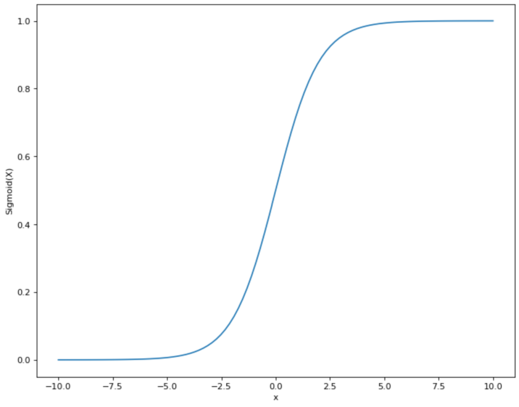
The functional equation of the sigmoid graph is as follows:
\(\) \[S(x) = \frac{1}{1+e^{-x}}\]
For our example:
\(\) \[P(\text{Purchase E-Bike})) = \frac{1}{1+e^{-(a + b_1 \cdot \text{Age})}}\]
This gives us a function that returns the probability of buying an e-bike and uses the person’s age as a variable. The graph for our example would then look something like this:

In practice, you often do not see the notation that we have used. Instead, the function is rearranged so that the actual regression equation becomes clear:
\(\) \[logit(P(\text{Kauf E-Bike}) = a + b_1 \cdot \text{Alter}\]
Ridge and Lasso Regression
With a high number of independent variables, an increased risk of overfitting quickly arises, as the model has too many regression parameters and therefore the risk increases when it simply memorizes structures from the training data set. For this reason, the following two subtypes of regression have been developed, which already contain regularization methods that are intended to prevent overfitting.
L1 – Regularization (Lasso)
L1 regularization, or Lasso (Least Absolute Shrinkage and Selection Operator), aims to minimize the absolute sum of all network parameters. This means that the model is penalized if the size of the parameters increases too much. This procedure can result in individual model parameters being set to zero during L1 regularization, which means that certain features in the data set are no longer taken into account. This results in a smaller model with less complexity, which only includes the most important features for the prediction.
Mathematically speaking, another term is added to the cost function. In our example, we assume a loss function with a mean squared error, in which the average squared deviation between the actual value from the data set and the prediction is calculated. The smaller this deviation, the better the model is at making the most accurate predictions possible.
For a model with the mean squared error as the loss function and an L1 regularization, the following cost function results:
\(\) \[J\left(\theta\right)=\frac{1}{m}\sum_{i=1}^{m}\left(y_i-\widehat{y_i}\right)^2+\lambda\sum_{j=1}^{n}\left|\theta_j\right|\]
- \(J\) is the cost function.
- \(\lambda\) is the regularization parameter that determines how strongly the regularization influences the error of the model.
- \(\sum_{j=1}^{n}\left|\theta_j\right|\) is the sum of all parameters of the model.
The model aims to minimize this cost function. So if the sum of the parameters increases, the cost function increases and there is an incentive to counteract this. \(\lambda\) can assume any positive value (>= 0). A value close to 0 stands for a less strong regularization, while a large value stands for a strong regularization. With the help of cross-validation, for example, different models with different degrees of regularization can be tested to find the optimal balance depending on the data.
Advantages of L1 Regularization:
- Feature Selection : By incentivizing the model to not let the size of the parameters increase too much, a few of the parameters are also set equal to 0. This removes certain features from the data set and automatically selects the most important features.
- Simplicity : A model with fewer features is easier to understand and interpret.
Disadvantages of L1 Regularization:
- Problems with Correlated Variables : If several variables in the data set are correlated with each other, Lasso tends to keep only one of the variables and set the other correlated variables to zero. This can result in information being lost that would have been present in the other variables.
L2 – Regularization (Ridge)
L2 regularization attempts to counter the problem of Lasso, i.e. the removal of variables that still contain information, by using the square of the parameters as the regularization term. Thus, it adds a penalty to the model that is proportional to the square of the parameters. As a result, the parameters do not go completely to zero but merely become smaller. The closer a parameter gets to zero in mathematical terms, the smaller its squared influence on the cost function becomes. This is why the model concentrates on other parameters before eliminating a parameter close to zero.
Mathematically, the ridge regularization for a model with the mean squared error as the loss function looks as follows:
\(\)\[J\left(\theta\right)=\frac{1}{m}\sum{\left(i=1\right)^m\left(y_i-\widehat{y_i}\right)^2}+\lambda\sum_{j=1}^{n}{\theta_j^2}\]
The parameters are identical to the previous formula with the difference that it is not the absolute value (\theta) that is added up, but the square.
Advantages of L2 Regularization:
- Stabilization : Ridge regularization ensures that the parameters react much more stably to small changes in the training data.
- Handling of Multicollinearity : With several correlated variables, L2 regularization ensures that these are considered together and not just one variable is kept in the model while the others are thrown out.
Disadvantages of L2 Regularization:
- No Feature Selection : Because Ridge does not set the parameters to zero, all features from the data set are retained in the model, which makes it less interpretable as more variables are considered.
Artificial Neural Networks
Artificial neural networks (ANN) are powerful tools for modeling complex relationships in data sets with many variables. Here, too, it must first be defined which variable or variables are to be predicted and which are to be used as input for the prediction. This is why neural networks are also categorized as structure-testing methods. They are based on the biological structure of the human brain. They are used to model and solve difficult computer-based problems and mathematical calculations.
In our brain, the information received from the sensory organs is recorded in so-called neurons. These process the information and then pass on an output that leads to a reaction in the body. Information processing does not just take place in a single neuron but in a multi-layered network of nodes.
In the artificial neural network, this biological principle is simulated and expressed mathematically. The neuron (also known as a node or unit) processes one or more inputs and calculates a single output from them. Three steps are carried out:
1. The various inputs \(x\) are multiplied by a weighting factor \(w\):
\(\) \[x_1 \rightarrow x_1 \cdot w_1, x_2 \rightarrow x_2 \cdot w_2 \]
The weighting factors determine how important an input is for the neuron to be able to solve the problem. If an input is very important, the value for the factor \(w\) increases. An unimportant input has a value of 0.
2. All weighted inputs of the neuron are added up. In addition, a bias \(b\) is added:
\(\) \[(x_1 \cdot w_1) + (x_2 \cdot w_2) + b \]
3. The result is then entered into a so-called activation function .
\(\) \[y = f((x_1 \cdot w_1) + (x_2 \cdot w_2) + b) \]
Various activation functions can be used. In many cases, this is the sigmoid function. This takes values and displays them in the range between 0 and 1:

This has the advantage for the neural network that all values that come from step 2 are within a specified smaller range. The sigmoid function therefore restricts values that can theoretically lie between (- ∞, + ∞) and maps them in the range between (0,1).
Now that we have understood what functions a single neuron has and what the individual steps within the node are, we can now turn to the artificial neural network. This is simply a collection of these neurons organized in different layers.
The information passes through the network in different layers:
- Input Layer : this is where the inputs for the model are entered and processed in the neurons before being passed on to the next layer.
- Hidden Layer(s) : One or more so-called hidden layers perform the actual information processing. The input from previous layers is weighted, processed in a neuron, and passed on to the next layer. This continues until the output layer is reached. As the calculations in this layer are not visible, but take place “hidden”, these collections of neurons are referred to as hidden layers.
- Output Layer : This layer follows on from the last hidden layer and takes over the outputs of the neurons. The results of the nodes in this layer contain the final result or decision of the neural network.
In the context of AI, it is often said that the models need to be trained and that a lot of data is required to deliver good results. But what exactly does this process mean for the artificial neural network?
From the data, the result is calculated for each data set that is produced when the network is run through and compared to see how good the result of the network is in comparison to the actual result from the data set. The aim is for the artificial neural network’s prediction to come ever closer to the actual result.
The neural network has an adjustment screw to bring the result closer to the actual outcome with each training step, namely the weighting of the outputs of the individual neurons. During the learning process, their weightings are constantly changed to alter the accuracy of the result. This means that each neuron decides which outputs of the previous neurons are important for its calculation and which are not. In the best-case scenario, this weight is consolidated with each new data set and the overall result becomes more accurate.
Here is a small example to illustrate this, which is of course not recommended for imitation. Three good friends are sitting next to you in math class. For every task that is calculated in class, you can ask all three of them to tell you their result because you are stuck yourself. All three of them are always happy to give you a number as a solution. Therefore, during the lessons (the training phase), you want to find out which of the three classmates usually has the best result.
For each task you calculate, you ask all three of them for their result and decide on one to compare it with the teacher’s result and find out which of the three classmates you can expect the best result from. Depending on the sub-area, you realize that one input is better than another. You therefore change the weightings in the training phase and refine them. In the exam, you will then ideally know exactly which of the three you need to turn to to get the correct result.
This is exactly what all neurons in the network do. During training, they are given a certain number of inputs, depending on how many neurons are “sitting” in the immediate vicinity. During training, they decide in each step which preliminary result is most suitable for them and then compare it with the actual result to determine whether they were correct. After the training, i.e. in the exam, they then know exactly which previous neurons are the most important.
What are the Advantages and Challenges of Multivariate Analysis?
The methods of multivariate analysis are powerful tools when working with large data sets and recognizing structures and correlations within them. Compared to univariate or bivariate analysis, it offers significantly more insight into the complex relationships within the data and thus creates a better understanding. However, the application of multivariate analysis also has some challenges, which we will discuss below.
The advantages of multivariate analysis include, for example:
- Better Understanding of Complex Relationships : By being able to analyze the relationships between multiple variables in more detail, even very complex relationships become quantifiable and apparent to researchers. These relationships are often not recognizable with simpler methods.
- Recognition of Latent Variables : Different multivariate methods can be used to identify so-called latent variables. These are not directly measurable constructs that can be derived from the observed data, such as empathy in psychology. Factor analysis can be used for this purpose, for example.
- Efficient Use of Data : By including several variables in the simultaneous analysis, the entire data set and the information it contains is better utilized and all recognizable structures are revealed.
In addition to these advantages, the use of multivariate methods also has some challenges that should be taken into account during implementation:
- High Model Complexity : The construction of multivariate models is often complex and requires a deep understanding of the underlying statistics in order to achieve optimal results. In addition, models that include several variables are also more difficult to interpret and validate, meaning that more work needs to go into these steps to achieve usable results.
- Data Quality Requirements : Data quality plays an even more important role in such complex methods to achieve reliable results. It must be ensured that the data set is complete, i.e. that there are no missing values, and that it is consistent, i.e. that it does not contain any incorrect values that could negatively influence the results. In addition, some methods, such as PCA, require the data to be standardized so that no erroneous dominant effects arise that are merely attributable to different scales.
- Intercorrelations : If the independent variables correlate strongly with each other, i.e. there is so-called multicollinearity in the data set, the stability and interpretability of the model can suffer as a result. These correlations must therefore be detected at an early stage and possibly only one of the correlated variables should remain in the data set.
- Overfitting : Due to the increasing number of variables Overfitting: The increasing number of variables and the higher model complexity also increase the risk of overfitting, i.e. the model memorizing specific properties of the data set and no longer concentrating on recognizing the basic structures. This leads to the model only providing poor predictions for new data.
- Computational Intensity : Many of the models presented are very computationally intensive, especially with large data sets, which means that not only do longer training times have to be accepted but more specialized hardware, such as graphics cards, may also be required.
Multivariate analysis offers many advantages when working with complex data sets and creating meaningful models. However, these also have to contend with some challenges, as more computing resources are required, for example, and the data quality must be very high to be able to make reliable predictions.
This is what you should take with you
- Multivariate analysis comprises methods that are designed to identify and quantify the relationship between several variables.
- Multivariate analyses are divided into structure-checking methods, which use a hypothesis as a basis, and structure-discovering methods, which recognize correlations completely independently.
- Multivariate analyses have the advantage that they can also recognize latent variables that are not directly present in the data set and also use the data set more efficiently, as all information and its correlations can be mapped.
- In this article, we have presented various multivariate analysis methods, such as artificial neural networks or principal component analysis.

What is Gibbs Sampling?
- 5. October 2024
Explore Gibbs sampling: Learn its applications, implementation, and how it's used in real-world data analysis.

What is a Bias?
- 27. July 2024
Unveiling Bias: Exploring its Impact and Mitigating Measures. Understand, recognize, and address bias in this insightful guide.

What is the Variance?
- 13. July 2024
Explore variance's role in statistics and data analysis. Understand how it measures data dispersion.

What is the Kullback-Leibler Divergence?
- 3. July 2024
Explore Kullback-Leibler Divergence, a vital metric in information theory and machine learning, and its applications.

What is the Maximum Likelihood Estimation?
- 29. June 2024
Unlocking insights: Understand Maximum Likelihood Estimation (MLE), a potent statistical tool for parameter estimation and data modeling.

What is the Variance Inflation Factor (VIF)?
- 18. May 2024
Learn how Variance Inflation Factor (VIF) detects multicollinearity in regression models for better data analysis.
Other Articles on the Topic of Multivariate Analysis
You can find an interesting article about Multivariate Analysis and other types on Medium.
Don't miss new articles!
We do not send spam! Read everything in our Privacy Policy .
Prüfe deinen Posteingang oder Spam-Ordner, um dein Abonnement zu bestätigen.

Niklas Lang
I have been working as a machine learning engineer and software developer since 2020 and am passionate about the world of data, algorithms and software development. In addition to my work in the field, I teach at several German universities, including the IU International University of Applied Sciences and the Baden-Württemberg Cooperative State University, in the fields of data science, mathematics and business analytics.
My goal is to present complex topics such as statistics and machine learning in a way that makes them not only understandable, but also exciting and tangible. I combine practical experience from industry with sound theoretical foundations to prepare my students in the best possible way for the challenges of the data world.
- Interview Questions
- Free Courses
- Career Guide
Recommended Data Science Courses

Data Science and Machine Learning from MIT
Earn an MIT IDSS certificate in Data Science and Machine Learning. Learn from MIT faculty, with hands-on training, mentorship, and industry projects.
PG in Data Science & Business Analytics from UT Austin
Advance your career with our 12-month Data Science and Business Analytics program from UT Austin. Industry-relevant curriculum with hands-on projects.
Multivariate Analysis Overview
What is multivariate analysis, the evolution of multivariate analysis, multivariate analysis: an overview, key applications of multivariate analysis, advantages and disadvantages of multivariate analysis, classification chart of multivariate techniques, comprehensive model building process, key multivariate techniques, model building process in multivariate analysis, multivariate analysis faqs, overview of multivariate analysis | what is multivariate analysis and model building process.

Multivariate Analysis (MVA) is a powerful statistical method that examines multiple variables to understand their impact on a specific outcome. This technique is crucial for analyzing complex data sets and uncovering hidden patterns across diverse fields such as weather forecasting, marketing, and healthcare. By exploring the relationships between several variables at once, MVA provides deeper insights and more accurate predictions, enhancing decision-making in data-driven industries. In this blog, we’ll explore the foundations, applications, and methods of multivariate analysis, highlighting its significance in modern data analysis.
Multivariate Analysis (MVA) is an essential statistical process used to understand the impact of multiple variables on a single outcome. This technique is fundamental in fields where complex interrelationships among data need to be studied, such as in weather forecasting where variables like temperature, humidity, and wind speed all influence weather conditions. Also, take up a Multivariate Time Series Forecasting In R to learn more about the concept.
Multivariate analysis has a rich history, beginning with John Wishart’s 1928 paper on sample covariance matrices. Over the decades, significant developments were made by statisticians like R.A. Fischer and Hotelling, initially applying these methods in psychology, education, and biology. The mid-20th century saw a technological boom with the advent of computers, expanding the application of multivariate analysis into new fields such as geology and meteorology. This period marked a shift from theoretical exploration to practical, computational applications.

Watch this youtube video for better understanding of Multivariate Analysis. It will provide you with an overview of the analysis.
The versatility of multivariate analysis is evident across various sectors:
- Healthcare: During the COVID-19 pandemic, multivariate analysis was crucial in forecasting disease spread and outcomes based on multiple health and environmental variables.
- Real Estate: Analysts use multivariate analysis to predict housing prices based on factors such as location, local infrastructure, and market conditions.
- Marketing: Techniques like conjoint analysis help determine consumer preferences and the trade-offs consumers make between different product attributes.
- The main advantage of multivariate analysis is that since it considers more than one factor of independent variables that influence the variability of dependent variables, the conclusion drawn is more accurate.
- The conclusions are more realistic and nearer to the real-life situation.
Disadvantages
- The main disadvantage of MVA includes that it requires rather complex computations to arrive at a satisfactory conclusion.
- Many observations for a large number of variables need to be collected and tabulated; it is a rather time-consuming process.
Selection of the appropriate multivariate technique depends upon-
a) Are the variables divided into independent and dependent classification?
b) If Yes, how many variables are treated as dependents in a single analysis?
c) How are the variables, both dependent and independent measured?
Multivariate analysis technique can be classified into two broad categories viz., This classification depends upon the question: are the involved variables dependent on each other or not?
If the answer is yes: We have Dependence methods. If the answer is no: We have Interdependence methods.
Dependence technique: Dependence Techniques are types of multivariate analysis techniques that are used when one or more of the variables can be identified as dependent variables and the remaining variables can be identified as independent.
Also Read: What is Big Data Analytics?
Model building in multivariate analysis involves several critical steps:
- Defining the Problem: Clearly defining what you need to solve or understand is the first step in multivariate analysis.
- Data Collection: Gathering adequate data for all variables considered relevant to the analysis.
- Data Preparation: Ensuring data cleanliness and proper format for analysis.
- Choosing the Right Model: Selecting a statistical model that fits the data and problem. This might include regression analysis, conjoint analysis, or discriminant analysis, depending on the complexity and nature of the problem.
- Model Testing and Validation: Rigorous testing to validate the model’s assumptions and its predictive power.
- Implementation and Monitoring: Applying the model in real-world scenarios and continually monitoring its effectiveness.
Below is a tabular overview of the primary multivariate analysis techniques, detailing their purposes and typical applications:
Building a model in multivariate analysis involves several critical steps:
- Defining Objectives: Clearly stating what you want to achieve with the analysis.
- Choosing Techniques: Selecting the appropriate statistical techniques based on the data and objectives.
- Assumption Testing: Checking assumptions like normality, homoscedasticity, linearity, and absence of multicollinearity.
- Model Estimation and Validation: Estimating the model parameters and validating the model through various diagnostic tests.
- Interpretation: Drawing conclusions from the model and applying these insights to make informed decisions.
Advantages Over Univariate and Bivariate Analysis
Unlike univariate or bivariate analysis, which examine one or two variables respectively, multivariate analysis provides a more comprehensive view by considering multiple variables simultaneously. This holistic approach leads to insights that are more detailed and closely aligned with the complexities of real-world scenarios.
Multivariate analysis is a powerful tool that, when applied correctly, can offer deep insights into complex data sets across various industries. It enables analysts to make more informed decisions, predict future trends, and optimize outcomes based on a thorough understanding of the interplay between multiple factors. For professionals looking to enhance their analytical skills, learning multivariate analysis through structured courses and hands-on practice is highly recommended.
If you are a beginner in the field of data science and wish to kick-start your career, taking up free online courses can help you grasp the introductory concepts in a comprehensive manner. Great Learning Academy offers a Data Science Foundations Free Online Course that can help you become job-ready. Some of the skills you will gain by the end of the course are linear programming, hands-on experience, and analytics landscape.
Three categories of multivariate analysis are: Cluster Analysis, Multiple Logistic Regression, and Multivariate Analysis of Variance.
Multivariate analysis is helpful in effectively minimizing the bias.
Multivariate refers to multiple dependent variables that result in one outcome. This means that a majority of our real-world problems are multivariate. For example, based on the season, we cannot predict the weather of any given year. Several factors play an important role in predicting the same. Such as, humidity, precipitation, pollution, etc.
There are several applications of multivariate analysis. It allows us to handle a huge dataset and discover hidden data structures that contribute to a better understanding and easy interpretation of data. There are various multivariate techniques that can be selected depending on the task at hand.
Multivariate analysis talks about two or more variables. It analyses which ones are correlated with a specific outcome. Whereas bivariate analysis talks about only two paired datasets and studies whether there is a relationship between them.
→ Explore this Curated Program for You ←

Data Cleaning in Python | What is Data Cleaning?

Apache Hadoop Tutorial |What is Apache Hadoop?

Mean Squared Error – Explained | What is Mean Square Error?

Understanding Distributions in Statistics

Introduction to Spectral Clustering

Apache Spark
IMAGES
VIDEO
COMMENTS
Multivariate analysis (MVA) is based on the principles of multivariate statistics.Typically, MVA is used to address situations where multiple measurements are made on each experimental unit and the relations among these measurements and their structures are important. [1] A modern, overlapping categorization of MVA includes: [1] Normal and general multivariate models and distribution theory
Researchers use multivariate procedures in studies that involve more than one dependent variable (also known as the outcome or phenomenon of interest), more than one independent variable (also known as a predictor) or both. Upper-level undergraduate courses and graduate courses in statistics teach multivariate statistical analysis.
Multivariate hypothesis testing is a statistical method used to determine whether there are significant differences between multiple groups across several variables simultaneously. This approach extends traditional hypothesis testing to situations where multiple dependent variables are analyzed together, allowing for a more comprehensive understanding of data relationships and group effects ...
Multivariate data analysis includes many complex computations and hence can be laborious. The analysis necessitates the collection and tabulation of a large number of observations for various variables. This process of observation takes a long time. (Also read: 15 Statistical Terms for Machine Learning) 7 Types of Multivariate Data Analysis
This problem can be thought of as the multivariate counterpart of the univariate hypothesis t-test. 9.1.1 Hotelling's T2 Test The most fundamental approach to signal detection is a mere generalization of the t-test, known as Hotelling's \(T^2\) test .
Multivariate analysis has particularly enjoyed a traditional stronghold in the field of behavioural sciences like psychology, psychiatry and allied fields because of the complex nature of the discipline. Conclusion. Multivariate analysis is one of the most useful methods to determine relationships and analyse patterns among large sets of data.
There are indeed also nonparametric procedures, mainly devoted to the analysis of independence or association among variables and to the multivariate extension of classical nonparametric tests of hypothesis, such as the sign test, the rank sum test, the Kruskal-Wallis test, the Kendall and Spearman tests, and similar.
STAT 542: Multivariate Analysis Spring 2021 Lecture 11: Multiple hypothesis test Instructor: Yen-Chi Chen 11.1 Introduction The multiple hypothesis testing is the scenario that we are conducting several hypothesis tests at the same time. Suppose we have ntests, each leads to a p-value. So we can view the 'data' as P 1; ;P n 2[0;1], where P
Multivariate analysis comprises methods that are designed to identify and quantify the relationship between several variables. Multivariate analyses are divided into structure-checking methods, which use a hypothesis as a basis, and structure-discovering methods, which recognize correlations completely independently.
Key Applications of Multivariate Analysis. The versatility of multivariate analysis is evident across various sectors: Healthcare: During the COVID-19 pandemic, multivariate analysis was crucial in forecasting disease spread and outcomes based on multiple health and environmental variables. Real Estate: Analysts use multivariate analysis to predict housing prices based on factors such as ...