hypothesis testing binomial distribution example

Hypothesis Testing with the Binomial Distribution

Contents Toggle Main Menu 1 Hypothesis Testing 2 Worked Example 3 See Also

Hypothesis Testing

To hypothesis test with the binomial distribution, we must calculate the probability, $p$, of the observed event and any more extreme event happening. We compare this to the level of significance $\alpha$. If $p>\alpha$ then we do not reject the null hypothesis. If $p<\alpha$ we accept the alternative hypothesis.

Worked Example

A coin is tossed twenty times, landing on heads six times. Perform a hypothesis test at a $5$% significance level to see if the coin is biased.

First, we need to write down the null and alternative hypotheses. In this case

The important thing to note here is that we only need a one-tailed test as the alternative hypothesis says “in favour of tails”. A two-tailed test would be the result of an alternative hypothesis saying “The coin is biased”.

We need to calculate more than just the probability that it lands on heads $6$ times. If it landed on heads fewer than $6$ times, that would be even more evidence that the coin is biased in favour of tails. Consequently we need to add up the probability of it landing on heads $1$ time, $2$ times, $\ldots$ all the way up to $6$ times. Although a calculation is possible, it is much quicker to use the cumulative binomial distribution table. This gives $\mathrm{P}[X\leq 6] = 0.058$.

We are asked to perform the test at a $5$% significance level. This means, if there is less than $5$% chance of getting less than or equal to $6$ heads then it is so unlikely that we have sufficient evidence to claim the coin is biased in favour of tails. Now note that our $p$-value $0.058>0.05$ so we do not reject the null hypothesis. We don't have sufficient evidence to claim the coin is biased.

But what if the coin had landed on heads just $5$ times? Again we need to read from the cumulative tables for the binomial distribution which shows $\mathrm{P}[X\leq 5] = 0.021$, so we would have had to reject the null hypothesis and accept the alternative hypothesis. So the point at which we switch from accepting the null hypothesis to rejecting it is when we obtain $5$ heads. This means that $5$ is the critical value .

Selecting a Hypothesis Test

Binomial Distribution: Hypothesis Testing

We welcome your feedback, comments and questions about this site or page. Please submit your feedback or enquiries via our Feedback page.

Numbers and Quantities

Statistics and Probability

Video Crash Courses

Junior Math

Math Essentials

Tutor-on-Demand

Encyclopedia

Digital Tools

How to Do Hypothesis Testing with Binomial Distribution

A hypothesis test has the objective of testing different results against each other. You use them to check a result against something you already believe is true. In a hypothesis test, you’re checking if the new alternative hypothesis  H A would challenge and replace the already existing null hypothesis  H 0 .

Hypothesis tests are either one-sided or two-sided. In a one-sided test, the alternative hypothesis is left-sided with p < p 0 or right-sided with p > p 0 . In a two-sided test, the alternative hypothesis is p ≠ p 0 . In all three cases, p 0 is the pre-existing probability of what you’re comparing, and p is the probability you are going to find.

Note! In hypothesis testing, you calculate the alternative hypothesis to say something about the null hypothesis.

Hypothesis Testing Binomial Distribution

For example, you would have a reason to believe that a high observed value of p , makes the alternative hypothesis H a : p > p 0 seem reasonable.

There is a drug on the market that you know cures 8 5 % of all patients. A company has come up with a new drug they believe is better than what is already on the market. This new drug has cured 92 of 103 patients in tests. Determine if the new drug is really better than the old one.

This is a classic case of hypothesis testing by binomial distribution. You now follow the recipe above to answer the task and select 5 % level of significance since it is not a question of medication for a serious illness.

The alternative hypothesis in this case is that the new drug is better. The reason for this is that you only need to know if you are going to approve for sale and thus the new drug must be better:

This result indicates that there is a 1 3 . 6 % chance that more than 92 patients would be cured with the old medicine.

so H 0 cannot be rejected. The new drug does not enter the market.

If the p value had been less than the level of significance, that would mean that the new drug represented by the alternative hypothesis is better, and that you are sure of this with statistical significance.

Professor McCarthy Statistics

Mat 150 bmcc, 10. hypothesis testing: p-values, exact binomial test, simple one-sided claims about proportions, the following 8 videos (run times vary from 2 to 8 minutes) will help you with your blackboard homework on this unit..

Please scroll down past these homework videos for an in depth explanation of Hypothesis Testing & P-values.

Question 2 and 3.

See Questions 4, 5, and 6, towards the bottom of this page for R scripts to calculate the p-value and a barplot for simple claims about proportions.

There are 2 videos at the end of Question 1 below.

A hypothesis is a claim about a population.

Examples of hypotheses:

• Claim: more than 60% of students like math.
• Claim: the mean weight of cats is less than 9 pounds

We test a claim by taking a sample from the population. If the data from the sample agrees with (or supports ) the claim, we say the data provides evidence that the claim is true.

• Claim : more than 60% of students like math.  $\rho > 60\%$ Data : If in a sample of 10 students 8 of them like math, the sample supports the claim because $\dfrac{8}{10} = 80\% > 60\%$. If 9 of the 10 liked math, the sample would provide even stronger support because 90% > 80% > 60%. If 6 of the 10 liked math, that data doesn’t support the claim since $\dfrac{6}{10} = 60\%$ is not more than 60%.
• Claim : the mean weight of cats is less than 9 pounds.  $\mu < 9 \text{ pounds }$ Data : If in a sample of 30 cats the mean weight was 8 pounds, the sample supports the claim because 8 pounds < 9 pounds. If in that sample the mean weight was 6 pounds, it would provide even stronger support of the claim because 6 pounds < 8 pounds < 9 pounds.

If the data from the sample supports the claim we can conduct a formal hypothesis test to determine if the sample provides statistically significant evidence that the claim is true.

After Question 7 (below) is a section on how to report the results of a hypothesis test .

p-value method of hypothesis testing

The p-value concept is difficult to understand at first. My suggestion is to read these definitions and descriptions. Then read through the first two or three Questions and their solutions. Then read these definitions again.

Definition . The sample used in the hypothesis test is called the test-sample .

Definition . The p-value is the maximum probability of getting a sample that provides as much support for the claim as the test-sample if we assume that the claim is false.

Note. “ as much support ” means the same or stronger support.

So, if the p-value is small, it would be very unlikely for us to get a sample which provides as much support for the claim being true, as the test-sample does, if the claim were false. So, if the p-value is small, the test-sample provides good evidence that the claim wasn’t false. So, a small p-value indicates the test-sample should be considered significant (strong) evidence that the claim is true.

WARNING!!! When we calculate a p-value it is with respect to a mathematical model of the “experiment”. The better the  model represents the experimental design, the sampling method, etc., the more relevant will be the p-value. Think about it. Unless the model faithfully represents the experiment, the p-value we calculate will tell us nothing meaningful. For more on this, please read the section, in Question 1 below, called: Important aside about mathematical models.

General algorithm to calculate the p-value:

If the claim is false, the maximum probability of getting a sample which supports the claim happens if the claim is false by the smallest amount possible. Think: little lies are difficult to detect.

So, to calculate the p-value we assume the claim is false by the smallest amount possible and then we calculate the probability of getting a sample that provides as much support as the test-sample.

How small does the p-value have to be in order for it indicate that the test-sample provides significant (strong) evidence that the claim is true?

Definition . If the p-value is smaller than a number called the level of significance , denoted $\alpha$, we say the sample provides statistically significant (strong) evidence that the claim is true.

Unless otherwise noted, in these notes we will always assume that $\alpha = 0.05$ as that is the most common value for  $\alpha$.

Type I and type II errors

Type I and type II errors . The definition of the  p-value is often given in terms of a concept called a type I error . A type I error is when a false claim is accepted as true. A type II error is when a true claim is rejected as false  1 .

We can define the p-value as: the maximum probability of making type I error, if we are willing to accept the claim as true whenever we get a sample that provides as much support as the test-sample.

Important notes about p-values

• Since p-values are a probability we always have $0 \leq \text{ p-value } \leq 1$.
• A small p-value doesn’t mean the claim is true, or even likely to be true .
• A large p-value means the data in the sample should not be reported as evidence of the claim being true.

The p-value method of hypothesis testing is probably the most common way to test a claim. It also is probably the most misunderstood concept in statistics.

The best way to understand the concept of a p-value is to learn how to calculate the p-value for a simple claim where the mathematics is not too difficult: the exact binomial test (see below). Other types of claims will have more complicated ways of calculating the p-value, but the meaning of the p-value doesn’t change.

P-value method of hypothesis testing for simple one-sided claims about a proportion. The Exact Binomial Test

A simple one-sided claim about a proportion is a claim that a proportion is greater than some percent or less than some percent.

The symbol for proportion is $\rho$.

The name of the hypothesis test that we use for this situation is “ the exact binomial test “.  Binomial because we use the binomial distribution. Exact because we don’t approximate the binomial distribution by a continuous distribution.

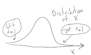
Note. Generally speaking, we test one-sided claims with one-tailed tests. The term “one-tailed” comes from the p-value being the area in one of the “tails” of the distribution.  See Figures below and the Figures accompanying the answers to Questions 1 through 6.

Question 1. 

Using the p-value method of hypothesis testing test the following claim at the $\alpha = 0.05$ significance level.

• Claim: More than 60% of students are STEM majors.
• Data:  In a sample of 10 students 8 of them are STEM majors.

Answer to Question 1. (Also, see video below).

• $n = $ the size of our sample, so $n = 10$.
• $X = $ the random variable that counts how many of the students in such samples ($n = 10$) are stem majors. $X(\text{our sample}) = 8$
• $\rho = $ “the true proportion of students in the population who are STEM majors”.

The sample’s proportion $\hat{p}$ of STEM majors is $$\hat{p} = \dfrac{X(\text{our sample})}{n} = \dfrac{8}{10} = 80\%$$ which supports our claim because $80\% > 60\%$.

Since the sample supports the claim, we conduct the hypothesis test and calculate the p-value.

In a formal hypothesis test we write the alternative and null hypotheses at the start of the problem. For us, $H_A$ (the alternative hypothesis) will always be the claim and $H_0$ (the null hypothesis) will always be the assumption for the parameters that we will use for our p-value calculation (basically that the claim is false in the smallest way possible):

$\text{(claim) } \ H_A: \rho > 60\%$ $\text{(null) } \ H_0: \rho = 60\%$

Important aside about mathematical models. For simple claims about a proportions, like in Question 1, we model the sampling process as a Bernoulli process having a binomial distribution. When we calculate a p-value it is with respect to the model, not to the actual experiment. The closer the  experimental design is  is to the model, the more relevant will be the p-value. Think about it. Suppose we have some real-life claim that we are testing. To save money, we could just make up the data and calculate the p-value; or we could collect the data in a sloppy manner, or make a mess of the data in a million ways; but what would a p-value based on such data tell us about the real world? Absolutely nothing.

T o calculate the p-value we assume the claim is false by the smallest amount possible and then we calculate the probability of getting a sample that provides as much support as the test-sample.

$X(\text{test-sample}) = 8$ so samples that provide as much support are samples which satisfy $X = 8, 9$, or $10$.

$$\text{p-value} = P(X \geq 8 \ \mid \rho = 60\%)$$

Notation.   $P(X \geq 8 \ \mid \rho = 60\%)$ means:

$P(X \geq 8)$ assuming that $\rho = 60\%$

Note. The assumption that $\rho = 60\%$ is the null hypothesis $H_0$. Also, see  footnote  2 on $P(A\mid B)$ and Conditional Probability.

As mentioned above, we model our claim and the sampling process as being a Bernoulli process having a binomial distribution with n = 10 and $\rho = 60\%$.  Other types of claims and sampling methods will have different mathematical models and involve different types of distributions.

Recall the binomial distribution formula:

$$P(X = r) = nCr\ \rho^r \ (1 – \rho)^{n-r}$$

Substituting in $n = 10$ and $\rho = 60\%$ we finally, actually calculate the p-value:

$\text{p-value} = P(X \geq 8 \  \mid \rho = 60\%)$ $ = P(X = 8) + P(X=9) + P(X= 10) $ $ = 10C8\ (60\%)^8 \ (40\%)^{2} $ $+ 10C9\ (60\%)^9 \ (40\%)^{1} $ $+ 10C10\ (60\%)^{10} \ (40\%)^{0}$ $=0.1209324 + 0.04031078 + 0.006046618$ $ = 0.1672898$

So, the p-value = 0.1672898.

Statistical significance.   If the p-value is LESS THAN the significance level $\alpha$ we can report:

• the sample provides statistically significant evidence that the claim is true, or
• the result of the study is statistically significant.

Result. Since the

(p-value = .1672898)   >   ($\alpha = .05$)

the sample doesn’t provide statistically significant evidence that the claim is true (at the $\alpha = 0.05$ significance level).

Note . In the above calculation, $ P(X = 8) + P(X=9) + P(X= 10) $ are all done with the assumption that $\rho = 60\%$.

Extremely important geometric interpretation of the p-value See barplot Figure below

Here is the probability density barplot corresponding to the p-value calculated in Question 1, above:

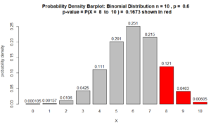
Figure for Question 1. The p-value is the area of the red bars.

For many statisticians, the above Figure is what explains the p-value. As the data from the sample provides more support, the p-value, which is the area of the red bars, decreases. See, for example, Question 2 below.

Note about the above barplot. The heights of the bars are probability densities and the areas of the bars are probabilities . Area = width $\times$ height. Since the bars’ widths are 1, the area of the bars are numerically equivalent to their height. In other words, the numbers on top of the bars are also probabilities. So, for example $P(X=8) = 0.121$.

So, we’ve finished Question 1.

Video showing how to solve Question 1 above (9:35):

Video for Question 1.

Continuation of above video showing solution to Question 2 below (3:34).

Video for Question 1 and 2 showing barplot.

Question 2: Redo the hypothesis test from Question 1, if $X(\text{our sample})$ had been 9, instead of 8. As in Question 1, the sample size is $n =10$ and the level of significance to be used is $\alpha = 0.05$.

Answer to Question 2:

• $X = $ the random variable that counts how many of the students in such samples are stem majors. $X(\text{our sample}) = 9$

The sample’s proportion $\hat{p}$ of STEM majors is $$\hat{p} = \dfrac{X(\text{our sample})}{n} = \dfrac{9}{10} = 90\%$$ which supports our claim because $80\% > 60\%$.

$\text{p-value} = P(X \geq 9 \  \mid \rho = 60\%)$ $ = P(X=9) + P(X= 10) $ $+ 10C9\ (60\%)^9 \ (40\%)^{1} $ $+ 10C10\ (60\%)^{10} \ (40\%)^{0}$ $= 0.04031078 + 0.006046618$ $ = 0.0463574$

which indicates statistical significance because 0.0463574 < 0.05. Also, see Figure below.

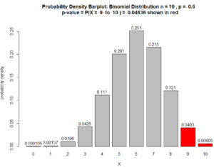
Figure for Question 2. The p-value is the area of the red bars.

Question 3. 

• Claim: Less than 60% of students are STEM majors.
• Data:  In a sample of 10 students 2 of them are STEM majors.

Answer to Question 3 .

• $X = $ the random variable that counts how many of the students in such samples are stem majors. $X(\text{our sample}) = 2$

The sample’s proportion $\hat{p}$ of STEM majors is $$\hat{p} = \dfrac{X(\text{our sample})}{n} = \dfrac{2}{10} = 20\%$$ which supports our claim because $20\% < 60\%$.

$\text{(claim) } \ H_A: \rho < 60\%$ $\text{(null) } \ H_0: \rho = 60\%$

$\text{p-value} = P(X \leq 2 \  \mid \rho = 60\%)$ $ = P(X=0) + P(X= 1) + P(X= 2) $ $+ 10C0\ (60\%)^0 \ (40\%)^{10} $ $+ 10C1\ (60\%)^1 \ (40\%)^{9}$ $+ 10C2\ (60\%)^2\ (40\%)^{8}$ $= 0.0001048576 +  0.001572864 +  0.010616832$ $ = 0.01229$

which indicates statistical significance because the

(p-value = .01229)   <   ($\alpha = 0.05$)

Also, see Figure below.

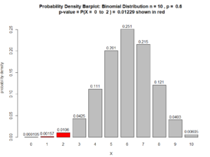
Figure for Question 3. The p-value is the area of the red bars.

Question 4. 

• Claim: Less than 49% of children play baseball.
• Data:  In a sample of 12 children 3 of them play baseball.

Answer to Question 4 .

• $n = $ the size of our sample, so $n = 12$.
• $X = $ the random variable that counts how many of the children in such samples are baseball players. $X(\text{our sample}) = 3$
• $\rho = $ “the true proportion of children in the population who play baseball”.

The sample’s proportion $\hat{p}$ of baseball players is $$\hat{p} = \dfrac{X(\text{our sample})}{n} = \dfrac{3}{12} = 25\%$$ which supports our claim because $25\% < 49\%$.

$\text{(claim) } \ H_A: \rho < 49\%$ $\text{(null) } \ H_0: \rho = 49\%$

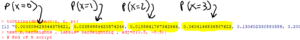
$\text{p-value} = P(X \leq 3 \  \mid \rho = 49\%)$ $ = P(X=0) + P(X= 1) + P(X= 2) + P(X=3) $ $+ 12C0\ (49\%)^0 \ (51\%)^{12} $ $+ 12C1\ (49\%)^1 \ (51\%)^{11}$ $+ 10C2\ (49\%)^2\ (51\%)^{10}$ $+ 10C3\ (49\%)^3\ (51\%)^{9}$ $= 0.000309629344375621 $ $+ 0.00356984420574246 $ $+ 0.0188641767342666$ $+ 0.0604146836587622$ $ = 0.08316$

which indicates NO statistical significance because the

(p-value = .08316)   >   ($\alpha = 0.05$)

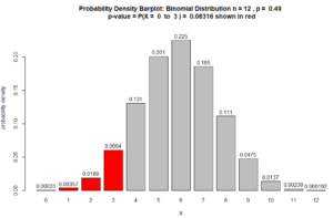
Figure for Question 4. The p-value is the area of the red bars.

Here is the R script used to create the above barplot.

The above script also outputs the distribution of $X$ to the “R Console” window:

Question 5. 

• Claim: More than 55% of children play baseball.
• Data:  In a sample of 12 children 10  of them play baseball.

Answer to Question 5 .

• $X = $ the random variable that counts how many of the children in such samples are baseball players. $X(\text{our sample}) = 10$

The sample’s proportion $\hat{p}$ of baseball players is $$\hat{p} = \dfrac{X(\text{our sample})}{n} = \dfrac{10}{12} = 83.3\%$$ which supports our claim because $83.3\%  > 55\%$.

$\text{(claim) } \ H_A: \rho > 55\%$ $\text{(null) } \ H_0: \rho = 55\%$

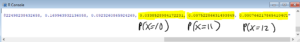
$\text{p-value} = P(X \geq 10 \  \mid \rho = 55\%)$ $ = P(X=10) + P(X= 11) + P(X= 12) $ $+ 12C10\ (55\%)^{10} \ (45\%)^{2} $ $+ 12C11\ (55\%)^{11} \ (45\%)^{1}$ $+ 12C12\ (55\%)^{12}\ (45\%)^{0}$ $= 0.0338528984172231$ $+ 0.00752286631493849$ $+ 0.000766217865410401$ $ = 0.04214$

which indicates the sample provides statistically significant evidence that the claim is true because the

(p-value = .04214)   <   ($\alpha = 0.05$)

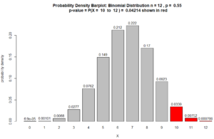
Figure for Question 5. The p-value is the area of the red bars.

Question 6. 

• Claim: More than 51% of children like chocolate.
• Data:  In a sample of 200 children 115  of them like chocolate.

Answer to Question 6 .

• $n = $ the size of our sample, so $n = 200$.
• $X = $ the random variable that counts how many of the children in such samples like chocolate. $X(\text{our sample}) = 115$
• $\rho = $ “the true proportion of children that like chocolate”.

The sample’s proportion $\hat{p}$ of children who like chocolate is $$\hat{p} = \dfrac{X(\text{our sample})}{n} = \dfrac{115}{200} = 57.5\%$$ which supports our claim because $57.5\%  > 51\%$.

$\text{(claim) } \ H_A: \rho > 51\%$ $\text{(null) } \ H_0: \rho = 51\%$

(The following calculation was too long to be done by hand. So I used R.)

$\text{p-value} = P(X \geq 115 \  \mid \rho = 51\%)$ $ = P(X=115) + P(X= 116) + \cdots +  P(X= 200) $ $+ 200C115\ (51\%)^{115} \ (49\%)^{85} $ $+ 200C116\ (51\%)^{116} \ (49\%)^{84}$ $\vdots$ $+ 200C200\ (51\%)^{200}\ (49\%)^{0}$ $= 0.010427568 $ $+ 0.007952763$ $\vdots$ $+ 3.266143\times 10^{-59}$ $ = 0.0383$

(p-value = .0383)   <   ($\alpha = .05$)

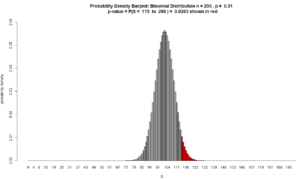
Figure for Question 6. The p-value is the area of the red bars.

Here is the R script used to create the above barplot. Since the bars are very thin, if we put numbers on top of them, the result will be a mess. So, this script omits the numbers on top of the bars.

If we just want to calculate the p-value, the script is much simpler:

Question 7. 

• Data:  In a sample of 200 children 100  of them like chocolate.

Answer to Question 7 .

• $X = $ the random variable that counts how many of the children in such samples like chocolate. $X(\text{our sample}) = 100$

The sample’s proportion $\hat{p}$ of children who like chocolate is $$\hat{p} = \dfrac{X(\text{our sample})}{n} = \dfrac{100}{200} = 50\%$$ which doesn’t support our claim.

The data is contrary to the claim, so we don’t have to calculate the p-value.

End of Question 7.

How to report these results in a scientific paper.

Each journal has its own style for how authors should report their results.

If the sample provided statistical significance , like in Question 6, the authors might write  something like:

More than 51% of children like chocolate (p = .0383, exact binomial test).

In our survey of 200 children, 57.5% liked chocolate, suggesting more than 51% of children like chocolate (p = .0308, exact binomial test).

The author’s won’t say they did a hypothesis test. They will often state the claim as if it were a fact (even though it isn’t). When they put the p-value they typically leave off the leading zero, so 0.0383 becomes .0383. Also, rather than write p-value, authors typically just write p. The authors won’t usually say that the results are statistically significant: the p-value being less than 0.05 indicates that. Finally, authors should name the type of hypothesis test that they used. In these examples the exact binomial test was used.

If the sample failed to provide statistical significance , for example, if in Question 6 we had $X = 104$, so that $\hat{p} = \dfrac{104}{200} = 52\%$, the p-value would be:

$$\text{p-value } = P(X \geq 104 \mid \rho = 51\%)  = .4162$$

If the authors wanted to include this inconclusive result in their paper, they might write something like:

As to the belief that more than 51% of children like chocolate: in our survey of 200 children, 52% said they liked chocolate, which not statistically significant (p = .4162, exact binomial test).

Based on our experiences with children, we expected that more than 51% of children would like chocolate: in our survey of 200 children, 52% said they liked chocolate, however this was not statistically significant (exact binomial test).

If the sample provided evidence contrary to the claim , like in Question 7 where we had $X = 100$ so that $\hat{p} = \dfrac{100}{200} = 50\%$  we wouldn’t bother to calculate the p-value (since the sample doesn’t support the claim).

It the authors wanted to include this contrary result, the authors might write something like:

We had thought that more than 51% of children liked chocolate. However, when we surveyed 200 children we found that only 50% said they liked chocolate.

An interesting way to think about the p-value.

• In some sense, the p-value measures how gullible you need to be in order to accept the claim as true based on the data in a sample. So, a smaller p-value indicates you’d need to be less gullible to accept the claim.

How a p-value should be used in the real world

• If the p-value is small, your doubts about the claim being true should be based more on the experimental design, or on an improperly chosen model, or that the authors used the wrong type of hypothesis test; rather than on things like the sample size being too small, or that, due to chance, getting a misleading sample.  Note. A small sample size will often result in a large p-value.
• A small p-value doesn’t mean that the claim is true, or is even likely to be true.
• A large p-value doesn’t mean the  claim is false.
• A large p-value means the data in the sample should not be presented as evidence of the claim being true.
• Different scientific fields will use different levels of significance to determine if the p-value is small or large, and whether the study can be reported as being “statistically significant”. In these notes we will always use a level of significance of $\alpha = 0.05$ because that is the most  commonly used value.

If we have to decide whether to accept a claim as true, there are two ways we could make a mistake or error.

• Type I Error .  A type I error is when a false claim is accepted as true. Type I errors are made by people who are too trusting and gullible.
• Type II Error .  A type II error is when we fail to accept a true claim. Type II errors are made by people who are too cynical.

$P(A \mid B)$ is read as the “probability of A assuming B”.

Example . Suppose $X$ is a binomally distributed random variable with $n = 10$. If we write

$$P(X = 8 \mid \rho = 60\%)$$

what we mean is

“the probability that $X = 8$ assuming that $\rho = 60\%$”.

Applying the binomial distribution formula we get:

$P(X = 8 \mid \rho = 60\%)$ $= 10C8\, \rho^8 (1 – \rho)^2$ $= 10C8\, (.60)^8 (.40)^2 $ $= 0.1209324$

Same example continued . Since $n = 10$ we have: $$P(X \geq 9 \mid \rho = 60\%) = P(X = 9 \mid \rho = 60\%) + P(X = 10 \mid \rho = 60\%)$$ However, the above is a little bit long, so to save space, we might write: $$P(X \geq 9 \mid \rho = 60\%) = P(X = 9) + P(X = 10)$$ where, in the above,  $P(X = 9)$ means  $P(X = 9 \mid \rho = 60\%)$ and  $P(X = 10)$  means  $P(X = 10 \mid \rho = 60\%)$.

Conditional probability uses the same notation $P(A \mid B)$.

Definition of conditional probability:

$$P(A \mid B) =   \dfrac{P(A \cap B}{P(B)}$$

In words $P(A \mid B) = $ the probability that A occurs if we assume that B occurs.  The conditional probability $P(A \mid B)$ is read as the “probability of A given B” or the “probability of A assuming B”.

Example .  If S = likes to swim and H = likes to hike, then $P(S \mid H)$ is the probability that a person likes to swim if we know they like to hike.  $P(H \mid S)$ is the probability that a person likes to hike if we know they like to swim.

Need help with the Commons?

Email us at [email protected] so we can respond to your questions and requests. Please email from your CUNY email address if possible. Or visit our help site for more information:

• Terms of Service
• Accessibility
• Creative Commons (CC) license unless otherwise noted

9.3 Probability Distribution Needed for Hypothesis Testing

Earlier in the course, we discussed sampling distributions. Particular distributions are associated with various types of hypothesis testing.

The following table summarizes various hypothesis tests and corresponding probability distributions that will be used to conduct the test (based on the assumptions shown below):

Assumptions

When you perform a hypothesis test of a single population mean μ using a normal distribution (often called a z-test), you take a simple random sample from the population. The population you are testing is normally distributed , or your sample size is sufficiently large. You know the value of the population standard deviation , which, in reality, is rarely known.

When you perform a hypothesis test of a single population mean μ using a Student's t-distribution (often called a t -test), there are fundamental assumptions that need to be met in order for the test to work properly. Your data should be a simple random sample that comes from a population that is approximately normally distributed. You use the sample standard deviation to approximate the population standard deviation. (Note that if the sample size is sufficiently large, a t -test will work even if the population is not approximately normally distributed).

When you perform a hypothesis test of a single population proportion p , you take a simple random sample from the population. You must meet the conditions for a binomial distribution : there are a certain number n of independent trials, the outcomes of any trial are success or failure, and each trial has the same probability of a success p . The shape of the binomial distribution needs to be similar to the shape of the normal distribution. To ensure this, the quantities np and nq must both be greater than five ( n p > 5   n p > 5   and n q > 5   n q > 5   ). Then the binomial distribution of a sample (estimated) proportion can be approximated by the normal distribution with μ = p   μ = p   and σ = p q n σ = p q n . Remember that q = 1 - p q q = 1 - p q .

Hypothesis Test for the Mean

Going back to the standardizing formula we can derive the test statistic for testing hypotheses concerning means.

The standardizing formula cannot be solved as it is because we do not have μ, the population mean. However, if we substitute in the hypothesized value of the mean, μ 0 in the formula as above, we can compute a Z value. This is the test statistic for a test of hypothesis for a mean and is presented in Figure 9.3 . We interpret this Z value as the associated probability that a sample with a sample mean of X ¯ X ¯ could have come from a distribution with a population mean of H 0 and we call this Z value Z c for “calculated”. Figure 9.3 and Figure 9.4 show this process.

In Figure 9.3 two of the three possible outcomes are presented. X ¯ 1 X ¯ 1 and X ¯ 3 X ¯ 3 are in the tails of the hypothesized distribution of H 0 . Notice that the horizontal axis in the top panel is labeled X ¯ X ¯ 's. This is the same theoretical distribution of X ¯ X ¯ 's, the sampling distribution, that the Central Limit Theorem tells us is normally distributed. This is why we can draw it with this shape. The horizontal axis of the bottom panel is labeled Z and is the standard normal distribution. Z α 2 Z α 2 and -Z α 2 -Z α 2 , called the critical values , are marked on the bottom panel as the Z values associated with the probability the analyst has set as the level of significance in the test, (α). The probabilities in the tails of both panels are, therefore, the same.

Notice that for each X ¯ X ¯ there is an associated Z c , called the calculated Z, that comes from solving the equation above. This calculated Z is nothing more than the number of standard deviations that the hypothesized mean is from the sample mean. If the sample mean falls "too many" standard deviations from the hypothesized mean we conclude that the sample mean could not have come from the distribution with the hypothesized mean, given our pre-set required level of significance. It could have come from H 0 , but it is deemed just too unlikely. In Figure 9.3 both X ¯ 1 X ¯ 1 and X ¯ 3 X ¯ 3 are in the tails of the distribution. They are deemed "too far" from the hypothesized value of the mean given the chosen level of alpha. If in fact this sample mean it did come from H 0 , but from in the tail, we have made a Type I error: we have rejected a good null. Our only real comfort is that we know the probability of making such an error, α, and we can control the size of α.

Figure 9.4 shows the third possibility for the location of the sample mean, x _ x _ . Here the sample mean is within the two critical values. That is, within the probability of (1-α) and we cannot reject the null hypothesis.

This gives us the decision rule for testing a hypothesis for a two-tailed test:

This rule will always be the same no matter what hypothesis we are testing or what formulas we are using to make the test. The only change will be to change the Z c to the appropriate symbol for the test statistic for the parameter being tested. Stating the decision rule another way: if the sample mean is unlikely to have come from the distribution with the hypothesized mean we cannot accept the null hypothesis. Here we define "unlikely" as having a probability less than alpha of occurring.

P-Value Approach

An alternative decision rule can be developed by calculating the probability that a sample mean could be found that would give a test statistic larger than the test statistic found from the current sample data assuming that the null hypothesis is true. Here the notion of "likely" and "unlikely" is defined by the probability of drawing a sample with a mean from a population with the hypothesized mean that is either larger or smaller than that found in the sample data. Simply stated, the p-value approach compares the desired significance level, α, to the p-value which is the probability of drawing a sample mean further from the hypothesized value than the actual sample mean. A large p -value calculated from the data indicates that we should not reject the null hypothesis . The smaller the p -value, the more unlikely the outcome, and the stronger the evidence is against the null hypothesis. We would reject the null hypothesis if the evidence is strongly against it. The relationship between the decision rule of comparing the calculated test statistics, Z c , and the Critical Value, Z α , and using the p -value can be seen in Figure 9.5 .

The calculated value of the test statistic is Z c in this example and is marked on the bottom graph of the standard normal distribution because it is a Z value. In this case the calculated value is in the tail and thus we cannot accept the null hypothesis, the associated X ¯ X ¯ is just too unusually large to believe that it came from the distribution with a mean of µ 0 with a significance level of α.

If we use the p -value decision rule we need one more step. We need to find in the standard normal table the probability associated with the calculated test statistic, Z c . We then compare that to the α associated with our selected level of confidence. In Figure 9.5 we see that the p -value is less than α and therefore we cannot accept the null. We know that the p -value is less than α because the area under the p-value is smaller than α/2. It is important to note that two researchers drawing randomly from the same population may find two different P-values from their samples. This occurs because the P-value is calculated as the probability in the tail beyond the sample mean assuming that the null hypothesis is correct. Because the sample means will in all likelihood be different this will create two different P-values. Nevertheless, the conclusions as to the null hypothesis should be different with only the level of probability of α.

Here is a systematic way to make a decision of whether you cannot accept or cannot reject a null hypothesis if using the p -value and a preset or preconceived α (the " significance level "). A preset α is the probability of a Type I error (rejecting the null hypothesis when the null hypothesis is true). It may or may not be given to you at the beginning of the problem. In any case, the value of α is the decision of the analyst. When you make a decision to reject or not reject H 0 , do as follows:

• If α > p -value, cannot accept H 0 . The results of the sample data are significant. There is sufficient evidence to conclude that H 0 is an incorrect belief and that the alternative hypothesis , H a , may be correct.
• If α ≤ p -value, cannot reject H 0 . The results of the sample data are not significant. There is not sufficient evidence to conclude that the alternative hypothesis, H a , may be correct. In this case the status quo stands.
• When you "cannot reject H 0 ", it does not mean that you should believe that H 0 is true. It simply means that the sample data have failed to provide sufficient evidence to cast serious doubt about the truthfulness of H 0 . Remember that the null is the status quo and it takes high probability to overthrow the status quo. This bias in favor of the null hypothesis is what gives rise to the statement "tyranny of the status quo" when discussing hypothesis testing and the scientific method.

Both decision rules will result in the same decision and it is a matter of preference which one is used.

One and Two-tailed Tests

The discussion of Figure 9.3 - Figure 9.5 was based on the null and alternative hypothesis presented in Figure 9.3 . This was called a two-tailed test because the alternative hypothesis allowed that the mean could have come from a population which was either larger or smaller than the hypothesized mean in the null hypothesis. This could be seen by the statement of the alternative hypothesis as μ ≠ 100, in this example.

It may be that the analyst has no concern about the value being "too" high or "too" low from the hypothesized value. If this is the case, it becomes a one-tailed test and all of the alpha probability is placed in just one tail and not split into α/2 as in the above case of a two-tailed test. Any test of a claim will be a one-tailed test. For example, a car manufacturer claims that their Model 17B provides gas mileage of greater than 25 miles per gallon. The null and alternative hypothesis would be:

• H 0 : µ ≤ 25
• H a : µ > 25

The claim would be in the alternative hypothesis. The burden of proof in hypothesis testing is carried in the alternative. This is because failing to reject the null, the status quo, must be accomplished with 90 or 95 percent confidence that it cannot be maintained. Said another way, we want to have only a 5 or 10 percent probability of making a Type I error, rejecting a good null; overthrowing the status quo.

This is a one-tailed test and all of the alpha probability is placed in just one tail and not split into α/2 as in the above case of a two-tailed test.

Figure 9.6 shows the two possible cases and the form of the null and alternative hypothesis that give rise to them.

where μ 0 is the hypothesized value of the population mean.

Effects of Sample Size on Test Statistic

In developing the confidence intervals for the mean from a sample, we found that most often we would not have the population standard deviation, σ. If the sample size were less than 30, we could simply substitute the point estimate for σ, the sample standard deviation, s, and use the student's t -distribution to correct for this lack of information.

When testing hypotheses we are faced with this same problem and the solution is exactly the same. Namely: If the population standard deviation is unknown, and the sample size is less than 30, substitute s, the point estimate for the population standard deviation, σ, in the formula for the test statistic and use the student's t -distribution. All the formulas and figures above are unchanged except for this substitution and changing the Z distribution to the student's t -distribution on the graph. Remember that the student's t -distribution can only be computed knowing the proper degrees of freedom for the problem. In this case, the degrees of freedom is computed as before with confidence intervals: df = (n-1). The calculated t-value is compared to the t-value associated with the pre-set level of confidence required in the test, t α , df found in the student's t tables. If we do not know σ, but the sample size is 30 or more, we simply substitute s for σ and use the normal distribution.

Table 9.5 summarizes these rules.

A Systematic Approach for Testing a Hypothesis

A systematic approach to hypothesis testing follows the following steps and in this order. This template will work for all hypotheses that you will ever test.

• Set up the null and alternative hypothesis. This is typically the hardest part of the process. Here the question being asked is reviewed. What parameter is being tested, a mean, a proportion, differences in means, etc. Is this a one-tailed test or two-tailed test?

Decide the level of significance required for this particular case and determine the critical value. These can be found in the appropriate statistical table. The levels of confidence typical for businesses are 80, 90, 95, 98, and 99. However, the level of significance is a policy decision and should be based upon the risk of making a Type I error, rejecting a good null. Consider the consequences of making a Type I error.

Next, on the basis of the hypotheses and sample size, select the appropriate test statistic and find the relevant critical value: Z α , t α , etc. Drawing the relevant probability distribution and marking the critical value is always big help. Be sure to match the graph with the hypothesis, especially if it is a one-tailed test.

• Take a sample(s) and calculate the relevant parameters: sample mean, standard deviation, or proportion. Using the formula for the test statistic from above in step 2, now calculate the test statistic for this particular case using the parameters you have just calculated.
• The test statistic is in the tail: Cannot Accept the null, the probability that this sample mean (proportion) came from the hypothesized distribution is too small to believe that it is the real home of these sample data.
• The test statistic is not in the tail: Cannot Reject the null, the sample data are compatible with the hypothesized population parameter.
• Reach a conclusion. It is best to articulate the conclusion two different ways. First a formal statistical conclusion such as “With a 5 % level of significance we cannot accept the null hypotheses that the population mean is equal to XX (units of measurement)”. The second statement of the conclusion is less formal and states the action, or lack of action, required. If the formal conclusion was that above, then the informal one might be, “The machine is broken and we need to shut it down and call for repairs”.

All hypotheses tested will go through this same process. The only changes are the relevant formulas and those are determined by the hypothesis required to answer the original question.

This book may not be used in the training of large language models or otherwise be ingested into large language models or generative AI offerings without OpenStax's permission.

Want to cite, share, or modify this book? This book uses the Creative Commons Attribution License and you must attribute OpenStax.

Access for free at https://openstax.org/books/introductory-business-statistics-2e/pages/1-introduction

• Authors: Alexander Holmes, Barbara Illowsky, Susan Dean
• Publisher/website: OpenStax
• Book title: Introductory Business Statistics 2e
• Publication date: Dec 13, 2023
• Location: Houston, Texas
• Book URL: https://openstax.org/books/introductory-business-statistics-2e/pages/1-introduction
• Section URL: https://openstax.org/books/introductory-business-statistics-2e/pages/9-3-probability-distribution-needed-for-hypothesis-testing

© Dec 6, 2023 OpenStax. Textbook content produced by OpenStax is licensed under a Creative Commons Attribution License . The OpenStax name, OpenStax logo, OpenStax book covers, OpenStax CNX name, and OpenStax CNX logo are not subject to the Creative Commons license and may not be reproduced without the prior and express written consent of Rice University.

• school Campus Bookshelves
• menu_book Bookshelves
• perm_media Learning Objects
• login Login
• how_to_reg Request Instructor Account
• hub Instructor Commons
• Download Page (PDF)
• Download Full Book (PDF)
• Periodic Table
• Physics Constants
• Scientific Calculator
• Reference & Cite
• Tools expand_more
• Readability

selected template will load here

This action is not available.

8.1.3: Distribution Needed for Hypothesis Testing

• Last updated
• Save as PDF
• Page ID 10975

Earlier in the course, we discussed sampling distributions. Particular distributions are associated with hypothesis testing. Perform tests of a population mean using a normal distribution or a Student's \(t\)-distribution. (Remember, use a Student's \(t\)-distribution when the population standard deviation is unknown and the distribution of the sample mean is approximately normal.) We perform tests of a population proportion using a normal distribution (usually \(n\) is large or the sample size is large).

If you are testing a single population mean, the distribution for the test is for means :

\[\bar{X} - N\left(\mu_{x}, \frac{\sigma_{x}}{\sqrt{n}}\right)\]

The population parameter is \(\mu\). The estimated value (point estimate) for \(\mu\) is \(\bar{x}\), the sample mean.

If you are testing a single population proportion, the distribution for the test is for proportions or percentages:

\[P' - N\left(p, \sqrt{\frac{p-q}{n}}\right)\]

The population parameter is \(p\). The estimated value (point estimate) for \(p\) is \(p′\). \(p' = \frac{x}{n}\) where \(x\) is the number of successes and n is the sample size.

Assumptions

When you perform a hypothesis test of a single population mean \(\mu\) using a Student's \(t\)-distribution (often called a \(t\)-test), there are fundamental assumptions that need to be met in order for the test to work properly. Your data should be a simple random sample that comes from a population that is approximately normally distributed. You use the sample standard deviation to approximate the population standard deviation. (Note that if the sample size is sufficiently large, a \(t\)-test will work even if the population is not approximately normally distributed).

When you perform a hypothesis test of a single population mean \(\mu\) using a normal distribution (often called a \(z\)-test), you take a simple random sample from the population. The population you are testing is normally distributed or your sample size is sufficiently large. You know the value of the population standard deviation which, in reality, is rarely known.

When you perform a hypothesis test of a single population proportion \(p\), you take a simple random sample from the population. You must meet the conditions for a binomial distribution which are: there are a certain number \(n\) of independent trials, the outcomes of any trial are success or failure, and each trial has the same probability of a success \(p\). The shape of the binomial distribution needs to be similar to the shape of the normal distribution. To ensure this, the quantities \(np\) and \(nq\) must both be greater than five \((np > 5\) and \(nq > 5)\). Then the binomial distribution of a sample (estimated) proportion can be approximated by the normal distribution with \(\mu = p\) and \(\sigma = \sqrt{\frac{pq}{n}}\). Remember that \(q = 1 – p\).

In order for a hypothesis test’s results to be generalized to a population, certain requirements must be satisfied.

When testing for a single population mean:

• A Student's \(t\)-test should be used if the data come from a simple, random sample and the population is approximately normally distributed, or the sample size is large, with an unknown standard deviation.
• The normal test will work if the data come from a simple, random sample and the population is approximately normally distributed, or the sample size is large, with a known standard deviation.

When testing a single population proportion use a normal test for a single population proportion if the data comes from a simple, random sample, fill the requirements for a binomial distribution, and the mean number of successes and the mean number of failures satisfy the conditions: \(np > 5\) and \(nq > 5\) where \(n\) is the sample size, \(p\) is the probability of a success, and \(q\) is the probability of a failure.

Formula Review

If there is no given preconceived \(\alpha\), then use \(\alpha = 0.05\).

Types of Hypothesis Tests

• Single population mean, known population variance (or standard deviation): Normal test .
• Single population mean, unknown population variance (or standard deviation): Student's \(t\)-test .
• Single population proportion: Normal test .
• For a single population mean , we may use a normal distribution with the following mean and standard deviation. Means: \(\mu = \mu_{\bar{x}}\) and \(\\sigma_{\bar{x}} = \frac{\sigma_{x}}{\sqrt{n}}\)
• A single population proportion , we may use a normal distribution with the following mean and standard deviation. Proportions: \(\mu = p\) and \(\sigma = \sqrt{\frac{pq}{n}}\).
• It is continuous and assumes any real values.
• The pdf is symmetrical about its mean of zero. However, it is more spread out and flatter at the apex than the normal distribution.
• It approaches the standard normal distribution as \(n\) gets larger.
• There is a "family" of \(t\)-distributions: every representative of the family is completely defined by the number of degrees of freedom which is one less than the number of data items.

Basic Statistics in Criminology and Criminal Justice pp 197–223 Cite as

Steps in a Statistical Test: Using the Binomial Distribution to Make Decisions About Hypotheses

• David Weisburd 5 , 6 ,
• Chester Britt 7 ,
• David B. Wilson 5 &
• Alese Wooditch 8  
• First Online: 24 February 2021

1383 Accesses

When we Make Inferences to a population, we rely on a statistic in our sample to make a decision about a population parameter. At the heart of our decision is a concern with Type I error. Before we reject our null hypothesis, we want to be fairly confident that it is in fact false for the population we are studying. For this reason, we want the observed risk of a Type I error in a test of statistical significance to be as small as possible. The first stage in a test of statistical significance is to state one’s assumptions. The second stage is to select an appropriate sampling distribution. The third stage is to select a significance level, which determines the rejection region and the location of the critical values of the test. The fourth stage involves calculating a test statistic. Finally, a decision is made: the null hypothesis will be rejected if the test statistic falls within the rejection region. When such a decision can be made, the results are said to be statistically significant.

• Null hypothesis
• Criminal justice
• Binomial distribution
• Sampling frame
• Sampling distribution

This is a preview of subscription content, log in via an institution .

Buying options

• Available as PDF
• Read on any device
• Instant download
• Own it forever
• Available as EPUB and PDF
• Compact, lightweight edition
• Dispatched in 3 to 5 business days
• Free shipping worldwide - see info
• Durable hardcover edition

Tax calculation will be finalised at checkout

Purchases are for personal use only

Problem-oriented policing is an important approach to police work formulated by Herman Goldstein of the University of Wisconsin Law School. See Goldstein ( 1990 ).

The hot spots were first put in pairs of alike places, and then one of each pair was randomly allocated to receive the experimental intervention.

The inclusion of a correction factor will make it easier for you to reject the null hypothesis. One problem criminal justice scholars face in using a correction factor is that they often want to infer to populations that are beyond their sampling frame. For example, a study of police patrol at hot spots in a particular city may sample 50 of 200 hot spots in the city during a certain month. However, researchers may be interested in making inferences to hot spots generally in the city (not just those that exist in a particular month) or even to hot spots in other places. For those inferences, it would be misleading to adjust the test statistic based on the small size of the sampling frame. For a discussion of how to correct for sampling without replacement, see Levy and Lemeshow ( 1991 ).

Braga, A. A. (1998). Solving violent crime problems: An evaluation of the Jersey City Police Department’s pilot program to control violent places. Unpublished manuscript, Rutgers University, Newark, NJ.

Google Scholar  

Goldstein, H. (1990). Problem-oriented policing. New York: McGraw-Hill.

Levy, P. S., & Lemeshow, S. (1991). Sampling of populations: Methods and applications. New York: Wiley.

Download references

Author information

Authors and affiliations.

Department of Criminology, Law and Society, George Mason University, Fairfax, VA, USA

David Weisburd & David B. Wilson

Institute of Criminology, Faculty of Law, Hebrew University of Jerusalem, Jerusalem, Israel

David Weisburd

Iowa State University, Ames, IA, USA

Chester Britt

Department of Criminal Justice, Temple University, Philadelphia, PA, USA

Alese Wooditch

You can also search for this author in PubMed   Google Scholar

Electronic supplementary material

Datasets_and_syntax_esm (zip 1kb), rights and permissions.

Reprints and permissions

Copyright information

© 2020 Springer Nature Switzerland AG

About this chapter

Cite this chapter.

Weisburd, D., Britt, C., Wilson, D.B., Wooditch, A. (2020). Steps in a Statistical Test: Using the Binomial Distribution to Make Decisions About Hypotheses. In: Basic Statistics in Criminology and Criminal Justice. Springer, Cham. https://doi.org/10.1007/978-3-030-47967-1_8

Download citation

DOI : https://doi.org/10.1007/978-3-030-47967-1_8

Published : 24 February 2021

Publisher Name : Springer, Cham

Print ISBN : 978-3-030-47966-4

Online ISBN : 978-3-030-47967-1

eBook Packages : Law and Criminology Law and Criminology (R0)

Share this chapter

Anyone you share the following link with will be able to read this content:

Sorry, a shareable link is not currently available for this article.

Provided by the Springer Nature SharedIt content-sharing initiative

• Publish with us

Policies and ethics

• Find a journal
• Track your research

• school Campus Bookshelves
• menu_book Bookshelves
• perm_media Learning Objects
• login Login
• how_to_reg Request Instructor Account
• hub Instructor Commons
• Download Page (PDF)
• Download Full Book (PDF)
• Periodic Table
• Physics Constants
• Scientific Calculator
• Reference & Cite
• Tools expand_more
• Readability

selected template will load here

This action is not available.

10.4: Distribution Needed for Hypothesis Testing

• Last updated
• Save as PDF
• Page ID 100396

Earlier in the course, we discussed sampling distributions. Particular distributions are associated with hypothesis testing. Perform tests of a population mean using a normal distribution or a Student's \(t\)-distribution . (Remember, use a Student's \(t\)-distribution when the population standard deviation is unknown and the distribution of the sample mean is approximately normal.) We perform tests of a population proportion using a normal distribution (usually \(n\) is large or the sample size is large).

If you are testing a single population mean, the distribution for the test is for means :

\[\bar{X} - N\left(\mu_{x}, \frac{\sigma_{x}}{\sqrt{n}}\right)\]

The population parameter is \(\mu\). The estimated value (point estimate) for \(\mu\) is \(\bar{x}\), the sample mean.

If you are testing a single population proportion, the distribution for the test is for proportions or percentages:

\[ \hat{p} - N\left(p, \sqrt{\frac{p-q}{n}}\right)\]

The population parameter is \(p\). The estimated value (point estimate) for \(p\) is \( \hat{p} \). \( \hat{p} = \frac{x}{n}\) where \(x\) is the number of successes and n is the sample size.

Assumptions

When you perform a hypothesis test of a single population mean \(\mu\) using a Student's \(t\)-distribution (often called a \(t\)-test), there are fundamental assumptions that need to be met in order for the test to work properly. Your data should be a simple random sample that comes from a population that is approximately normally distributed. You use the sample standard deviation to approximate the population standard deviation. (Note that if the sample size is sufficiently large, a \(t\)-test will work even if the population is not approximately normally distributed).

When you perform a hypothesis test of a single population mean \(\mu\) using a normal distribution (often called a \(z\)-test), you take a simple random sample from the population. The population you are testing is normally distributed or your sample size is sufficiently large. You know the value of the population standard deviation which, in reality, is rarely known.

When you perform a hypothesis test of a single population proportion \(p\), you take a simple random sample from the population. You must meet the conditions for a binomial distribution which are: there are a certain number \(n\) of independent trials, the outcomes of any trial are success or failure, and each trial has the same probability of a success \(p\). The shape of the binomial distribution needs to be similar to the shape of the normal distribution. To ensure this, the quantities \(np\) and \(nq\) must both be greater than five \((np > 5\) and \(nq > 5)\). Then the binomial distribution of a sample (estimated) proportion can be approximated by the normal distribution with \(\mu = p\) and \(\sigma = \sqrt{\frac{pq}{n}}\). Remember that \(q = 1 – p\).

In order for a hypothesis test’s results to be generalized to a population, certain requirements must be satisfied.

When testing for a single population mean:

• A Student's \(t\)-test should be used if the data come from a simple, random sample and the population is approximately normally distributed, or the sample size is large, with an unknown standard deviation.
• The normal test will work if the data come from a simple, random sample and the population is approximately normally distributed, or the sample size is large, with a known standard deviation.

When testing a single population proportion use a normal test for a single population proportion if the data comes from a simple, random sample, fill the requirements for a binomial distribution, and the mean number of success and the mean number of failures satisfy the conditions: \(np > 5\) and \(nq > n\) where \(n\) is the sample size, \(p\) is the probability of a success, and \(q\) is the probability of a failure.

Formula Review

If there is no given preconceived \(\alpha\), then use \(\alpha = 0.05\).

Types of Hypothesis Tests

• Single population mean, known population variance (or standard deviation): Normal test .
• Single population mean, unknown population variance (or standard deviation): Student's \(t\)-test .
• Single population proportion: Normal test .
• For a single population mean , we may use a normal distribution with the following mean and standard deviation. Means: \(\mu = \mu_{\bar{x}}\) and \(\\sigma_{\bar{x}} = \frac{\sigma_{x}}{\sqrt{n}}\)
• A single population proportion , we may use a normal distribution with the following mean and standard deviation. Proportions: \(\mu = p\) and \(\sigma = \sqrt{\frac{pq}{n}}\).
• It is continuous and assumes any real values.
• The pdf is symmetrical about its mean of zero. However, it is more spread out and flatter at the apex than the normal distribution.
• It approaches the standard normal distribution as \(n\) gets larger.
• There is a "family" of \(t\)-distributions: every representative of the family is completely defined by the number of degrees of freedom which is one less than the number of data items.

Contributors

Barbara Illowsky and Susan Dean (De Anza College) with many other contributing authors. Content produced by OpenStax College is licensed under a Creative Commons Attribution License 4.0 license. Download for free at http://cnx.org/contents/[email protected] .