meta analysis type of research

An official website of the United States government

The .gov means it’s official. Federal government websites often end in .gov or .mil. Before sharing sensitive information, make sure you’re on a federal government site.

The site is secure. The https:// ensures that you are connecting to the official website and that any information you provide is encrypted and transmitted securely.

• Publications
• Account settings

Preview improvements coming to the PMC website in October 2024. Learn More or Try it out now .

• Advanced Search
• Journal List
• Front Physiol

Meta-Analytic Methodology for Basic Research: A Practical Guide

Nicholas mikolajewicz.

1 Faculty of Dentistry, McGill University, Montreal, QC, Canada

2 Shriners Hospital for Children-Canada, Montreal, QC, Canada

Svetlana V. Komarova

Associated data.

Basic life science literature is rich with information, however methodically quantitative attempts to organize this information are rare. Unlike clinical research, where consolidation efforts are facilitated by systematic review and meta-analysis, the basic sciences seldom use such rigorous quantitative methods. The goal of this study is to present a brief theoretical foundation, computational resources and workflow outline along with a working example for performing systematic or rapid reviews of basic research followed by meta-analysis. Conventional meta-analytic techniques are extended to accommodate methods and practices found in basic research. Emphasis is placed on handling heterogeneity that is inherently prevalent in studies that use diverse experimental designs and models. We introduce MetaLab , a meta-analytic toolbox developed in MATLAB R2016b which implements the methods described in this methodology and is provided for researchers and statisticians at Git repository ( https://github.com/NMikolajewicz/MetaLab ). Through the course of the manuscript, a rapid review of intracellular ATP concentrations in osteoblasts is used as an example to demonstrate workflow, intermediate and final outcomes of basic research meta-analyses. In addition, the features pertaining to larger datasets are illustrated with a systematic review of mechanically-stimulated ATP release kinetics in mammalian cells. We discuss the criteria required to ensure outcome validity, as well as exploratory methods to identify influential experimental and biological factors. Thus, meta-analyses provide informed estimates for biological outcomes and the range of their variability, which are critical for the hypothesis generation and evidence-driven design of translational studies, as well as development of computational models.

Introduction

Evidence-based medical practice aims to consolidate best research evidence with clinical and patient expertise. Systematic reviews and meta-analyses are essential tools for synthesizing evidence needed to inform clinical decision making and policy. Systematic reviews summarize available literature using specific search parameters followed by critical appraisal and logical synthesis of multiple primary studies (Gopalakrishnan and Ganeshkumar, 2013 ). Meta-analysis refers to the statistical analysis of the data from independent primary studies focused on the same question, which aims to generate a quantitative estimate of the studied phenomenon, for example, the effectiveness of the intervention (Gopalakrishnan and Ganeshkumar, 2013 ). In clinical research, systematic reviews and meta-analyses are a critical part of evidence-based medicine. However, in basic science, attempts to evaluate prior literature in such rigorous and quantitative manner are rare, and narrative reviews are prevalent. The goal of this manuscript is to provide a brief theoretical foundation, computational resources and workflow outline for performing a systematic or rapid review followed by a meta-analysis of basic research studies.

Meta-analyses can be a challenging undertaking, requiring tedious screening and statistical understanding. There are several guides available that outline how to undertake a meta-analysis in clinical research (Higgins and Green, 2011 ). Software packages supporting clinical meta-analyses include the Excel plugins MetaXL (Barendregt and Doi, 2009 ) and Mix 2.0 (Bax, 2016 ), Revman (Cochrane Collaboration, 2011 ), Comprehensive Meta-Analysis Software [CMA (Borenstein et al., 2005 )], JASP (JASP Team, 2018 ) and MetaFOR library for R (Viechtbauer, 2010 ). While these packages can be adapted to basic science projects, difficulties may arise due to specific features of basic science studies, such as large and complex datasets and heterogeneity in experimental methodology. To address these limitations, we developed a software package aimed to facilitate meta-analyses of basic research, MetaLab in MATLAB R2016b, with an intuitive graphical interface that permits users with limited statistical and coding background to proceed with a meta-analytic project. We organized MetaLab into six modules ( Figure 1 ), each focused on different stages of the meta-analytic process, including graphical-data extraction, model parameter estimation, quantification and exploration of heterogeneity, data-synthesis, and meta-regression.

General framework of MetaLab . The Data Extraction module assists with graphical data extraction from study figures. Fit Model module applies Monte-Carlo error propagation approach to fit complex datasets to model of interest. Prior to further analysis, reviewers have opportunity to manually curate and consolidate data from all sources. Prepare Data module imports datasets from a spreadsheet into MATLAB in a standardized format. Heterogeneity, Meta-analysis and Meta-regression modules facilitate meta-analytic synthesis of data.

In the present manuscript, we describe each step of the meta-analytic process with emphasis on specific considerations made when conducting a review of basic research. The complete workflow of parameter estimation using MetaLab is demonstrated for evaluation of intracellular ATP content in osteoblasts (OB [ATP] ic dataset) based on a rapid literature review. In addition, the features pertaining to larger datasets are explored with the ATP release kinetics from mechanically-stimulated mammalian cells (ATP release dataset) obtained as a result of a systematic review in our prior work (Mikolajewicz et al., 2018 ).

MetaLab can be freely accessed at Git repository ( https://github.com/NMikolajewicz/MetaLab ), and a detailed documentation of how to use MetaLab together with a working example is available in the Supporting materials .

Validity of Evidence in the Basic Sciences

To evaluate the translational potential of basic research, the validity of evidence must first be assessed, usually by examining the approach taken to collect and evaluate the data. Studies in the basic sciences are broadly grouped as hypothesis-generating and hypothesis-driven. The former tend to be small-sampled proof-of-principle studies and are typically exploratory and less valid than the latter. An argument can even be made that studies that report novel findings fall into this group as well, since their findings remain subject to external validation prior to being accepted by the broader scientific community. Alternatively, hypothesis-driven studies build upon what is known or strongly suggested by earlier work. These studies can also validate prior experimental findings with incremental contributions. Although such studies are often overlooked and even dismissed due to a lack of substantial novelty, their role in external validation of prior work is critical for establishing the translational potential of findings.

Another dimension to the validity of evidence in the basic sciences is the selection of experimental model. The human condition is near-impossible to recapitulate in a laboratory setting, therefore experimental models (e.g., cell lines, primary cells, animal models) are used to mimic the phenomenon of interest, albeit imperfectly. For these reasons, the best quality evidence comes from evaluating the performance of several independent experimental models. This is accomplished through systematic approaches that consolidate evidence from multiple studies, thereby filtering the signal from the noise and allowing for side-by-side comparison. While systematic reviews can be conducted to accomplish a qualitative comparison, meta-analytic approaches employ statistical methods which enable hypothesis generation and testing. When a meta-analysis in the basic sciences is hypothesis-driven, it can be used to evaluate the translational potential of a given outcome and provide recommendations for subsequent translational- and clinical-studies. Alternatively, if meta-analytic hypothesis testing is inconclusive, or exploratory analyses are conducted to examine sources of inconsistency between studies, novel hypotheses can be generated, and subsequently tested experimentally. Figure 2 summarizes this proposed framework.

Schematic of proposed hierarchy of translational potential in basic research.

Steps in Quantitative Literature Review

All meta-analytic efforts prescribe to a similar workflow, outlined as follows:

• Define primary and secondary objectives
• Determine breadth of question
• Construct search strategy: rapid or systematic search
• Screen studies and determine eligibility
• Extract data from relevant studies
• Collect relevant study-level characteristics and experi-mental covariates
• Evaluate quality of studies
• Estimate model parameters for complex relation-ships (optional)
• Compute appropriate outcome measure
• Evaluate extent of between-study inconsistency (heterogeneity)
• Perform relevant data transformations
• Select meta-analytic model
• Pool data and calculate summary measure and confidence interval
• Explore potential sources of heterogeneity (ex. biological or experimental)
• Subgroup and meta-regression analyses
• Interpret findings
• Provide recommendations for future work

Meta-Analysis Methodology

Search and selection strategies.

The first stage of any review involves formulating a primary objective in the form of a research question or hypothesis. Reviewers must explicitly define the objective of the review before starting the project, which serves to reduce the risk of data dredging, where reviewers later assign meaning to significant findings. Secondary objectives may also be defined; however, precaution must be taken as the search strategies formulated for the primary objective may not entirely encompass the body of work required to address the secondary objective. Depending on the purpose of a review, reviewers may choose to undertake a rapid or systematic review. While the meta-analytic methodology is similar for systematic and rapid reviews, the scope of literature assessed tends to be significantly narrower for rapid reviews permitting the project to proceed faster.

Systematic Review and Meta-Analysis

Systematic reviews involve comprehensive search strategies that enable reviewers to identify all relevant studies on a defined topic (DeLuca et al., 2008 ). Meta-analytic methods then permit reviewers to quantitatively appraise and synthesize outcomes across studies to obtain information on statistical significance and relevance. Systematic reviews of basic research data have the potential of producing information-rich databases which allow extensive secondary analysis. To comprehensively examine the pool of available information, search criteria must be sensitive enough not to miss relevant studies. Key terms and concepts that are expressed as synonymous keywords and index terms, such as Medical Subject Headings (MeSH), must be combined using Boolean operators AND, OR and NOT (Ecker and Skelly, 2010 ). Truncations, wildcards, and proximity operators can also help refine a search strategy by including spelling variations and different wordings of the same concept (Ecker and Skelly, 2010 ). Search strategies can be validated using a selection of expected relevant studies. If the search strategy fails to retrieve even one of the selected studies, the search strategy requires further optimization. This process is iterated, updating the search strategy in each iterative step until the search strategy performs at a satisfactory level (Finfgeld-Connett and Johnson, 2013 ). A comprehensive search is expected to return a large number of studies, many of which are not relevant to the topic, commonly resulting in a specificity of <10% (McGowan and Sampson, 2005 ). Therefore, the initial stage of sifting through the library to select relevant studies is time-consuming (may take 6 months to 2 years) and prone to human error. At this stage, it is recommended to include at least two independent reviewers to minimize selection bias and related errors. Nevertheless, systematic reviews have a potential to provide the highest quality quantitative evidence synthesis to directly inform the experimental and computational basic, preclinical and translational studies.

Rapid Review and Meta-Analysis

The goal of the rapid review, as the name implies, is to decrease the time needed to synthesize information. Rapid reviews are a suitable alternative to systematic approaches if reviewers prefer to get a general idea of the state of the field without an extensive time investment. Search strategies are constructed by increasing search specificity, thus reducing the number of irrelevant studies identified by the search at the expense of search comprehensiveness (Haby et al., 2016 ). The strength of a rapid review is in its flexibility to adapt to the needs of the reviewer, resulting in a lack of standardized methodology (Mattivi and Buchberger, 2016 ). Common shortcuts made in rapid reviews are: (i) narrowing search criteria, (ii) imposing date restrictions, (iii) conducting the review with a single reviewer, (iv) omitting expert consultation (i.e., librarian for search strategy development), (v) narrowing language criteria (ex. English only), (vi) foregoing the iterative process of searching and search term selection, (vii) omitting quality checklist criteria and (viii) limiting number of databases searched (Ganann et al., 2010 ). These shortcuts will limit the initial pool of studies returned from the search, thus expediting the selection process, but also potentially resulting in the exclusion of relevant studies and introduction of selection bias. While there is a consensus that rapid reviews do not sacrifice quality, or synthesize misrepresentative results (Haby et al., 2016 ), it is recommended that critical outcomes be later verified by systematic review (Ganann et al., 2010 ). Nevertheless, rapid reviews are a viable alternative when parameters for computational modeling need to be estimated. While systematic and rapid reviews rely on different strategies to select the relevant studies, the statistical methods used to synthesize data from the systematic and rapid review are identical.

Screening and Selection

When the literature search is complete (the date articles were retrieved from the databases needs to be recorded), articles are extracted and stored in a reference manager for screening. Before study screening, the inclusion and exclusion criteria must be defined to ensure consistency in study identification and retrieval, especially when multiple reviewers are involved. The critical steps in screening and selection are (1) removing duplicates, (2) screening for relevant studies by title and abstract, and (3) inspecting full texts to ensure they fulfill the eligibility criteria. There are several reference managers available including Mendeley and Rayyan, specifically developed to assist with screening systematic reviews. However, 98% of authors report using Endnote, Reference Manager or RefWorks to prepare their reviews (Lorenzetti and Ghali, 2013 ). Reference managers often have deduplication functions; however, these can be tedious and error-prone (Kwon et al., 2015 ). A protocol for faster and more reliable de-duplication in Endnote has been recently proposed (Bramer et al., 2016 ). The selection of articles should be sufficiently broad not to be dominated by a single lab or author. In basic research articles, it is common to find data sets that are reused by the same group in multiple studies. Therefore, additional precautions should be taken when deciding to include multiple studies published by a single group. At the end of the search, screening and selection process, the reviewer obtains a complete list of eligible full-text manuscripts. The entire screening and selection process should be reported in a PRISMA diagram, which maps the flow of information throughout the review according to prescribed guidelines published elsewhere (Moher et al., 2009 ). Figure 3 provides a summary of the workflow of search and selection strategies using the OB [ATP] ic rapid review and meta-analysis as an example.

Example of the rapid review literature search. (A) Development of the search parameters to find literature on the intracellular ATP content in osteoblasts. (B) PRISMA diagram for the information flow.

Data Extraction, Initial Appraisal, and Preparation

Identification of parameters to be extracted.

It is advised to predefine analytic strategies before data extraction and analysis. However, the availability of reported effect measures and study designs will often influence this decision. When reviewers aim to estimate the absolute mean difference (absolute effect), normalized mean difference, response ratio or standardized mean difference (ex. Hedges' g), they need to extract study-level means (θ i ), standard deviations ( sd (θ i )), and sample sizes ( n i ), for control (denoted θ i c , s d ( θ i c ) , and n i c ) and intervention (denoted θ i r , s d ( θ i r ) , and n i r ) groups, for studies i . To estimate absolute mean effect, only the mean ( θ i r ), standard deviation ( s d ( θ i r ) ) , and sample size ( n i r ) are required. In basic research, it is common for a single study to present variations of the same observation (ex. measurements of the same entity using different techniques). In such cases, each point may be treated as an individual observation, or common outcomes within a study can be pooled by taking the mean weighted by the sample size. Another consideration is inconsistency between effect size units reported on the absolute scale, for example, protein concentrations can be reported as g/cell, mol/cell, g/g wet tissue or g/g dry tissue. In such cases, conversion to a common representation is required for comparison across studies, for which appropriate experimental parameters and calibrations need to be extracted from the studies. While some parameters can be approximated by reviewers, such as cell-related parameters found in BioNumbers database (Milo et al., 2010 ) and equipment-related parameters presumed from manufacturer manuals, reviewers should exercise caution when making such approximations as they can introduce systematic errors that manifest throughout the analysis. When data conversion is judged to be difficult but negative/basal controls are available, scale-free measures (i.e., normalized, standardized, or ratio effects) can still be used in the meta-analysis without the need to convert effects to common units on the absolute scale. In many cases, reviewers may only be able to decide on a suitable effect size measure after data extraction is complete.

It is regrettably common to encounter unclear or incomplete reporting, especially for the sample sizes and uncertainties. Reviewers may choose to reject studies with such problems due to quality concerns or to employ conservative assumptions to estimate missing data. For example, if it is unclear if a study reports the standard deviation or standard error of the mean, it can be assumed to be a standard error, which provides a more conservative estimate. If a study does not report uncertainties but is deemed important because it focuses on a rare phenomenon, imputation methods have been proposed to estimate uncertainty terms (Chowdhry et al., 2016 ). If a study reports a range of sample sizes, reviewers should extract the lowest value. Strategies to handle missing data should be pre-defined and thoroughly documented.

In addition to identifying relevant primary parameters, a priori defined study-level characteristics that have a potential to influence the outcome, such as species, cell type, specific methodology, should be identified and collected in parallel to data extraction. This information is valuable in subsequent exploratory analyses and can provide insight into influential factors through between-study comparison.

Quality Assessment

Formal quality assessment allows the reviewer to appraise the quality of identified studies and to make informed and methodical decision regarding exclusion of poorly conducted studies. In general, based on initial evaluation of full texts, each study is scored to reflect the study's overall quality and scientific rigor. Several quality-related characteristics have been described (Sena et al., 2007 ), such as: (i) published in peer-reviewed journal, (ii) complete statistical reporting, (iii) randomization of treatment or control, (iv) blinded analysis, (v) sample size calculation prior to the experiment, (vi) investigation of a dose-response relationship, and (vii) statement of compliance with regulatory requirements. We also suggest that the reviewers of basic research studies assess (viii) objective alignment between the study in question and the meta-analytic project. This involves noting if the outcome of interest was the primary study objective or was reported as a supporting or secondary outcome, which may not receive the same experimental rigor and is subject to expectation bias (Sheldrake, 1997 ). Additional quality criteria specific to experimental design may be included at the discretion of the reviewer. Once study scores have been assembled, study-level aggregate quality scores are determined by summing the number of satisfied criteria, and then evaluating how outcome estimates and heterogeneity vary with study quality. Significant variation arising from poorer quality studies may justify study omission in subsequent analysis.

Extraction of Tabular and Graphical Data

The next step is to compile the meta-analytic data set, which reviewers will use in subsequent analysis. For each study, the complete dataset which includes parameters required to estimate the target outcome, study characteristics, as well as data necessary for unit conversion needs to be extracted. Data reporting in basic research are commonly tabular or graphical. Reviewers can accurately extract tabular data from the text or tables. However, graphical data often must be extracted from the graph directly using time consuming and error prone methods. The Data Extraction Module in MetaLab was developed to facilitate systematic and unbiased data extraction; Reviewers provide study figures as inputs, then specify the reference points that are used to calibrate the axes and extract the data ( Figures 4A,B ).

MetaLab data extraction procedure is accurate, unbiased and robust to quality of data presentation. (A,B) Example of graphical data extraction using MetaLab. (A) Original figure (Bodin et al., 1992 ) with axes, data points and corresponding errors marked by reviewer. (B) Extracted data with error terms. (C–F) Validation of MetaLab data-extraction module. (C) Synthetic datasets were constructed using randomly generated data coordinates and marker sizes. (D) Extracted values were consistent with true values evaluated by linear regression with the slope β slope , red line: line of equality. (E) Data extraction was unbiased, evaluated with distribution of percent errors between true and extracted values. E mean , E median , E min , and E max are mean, median, minimum, and maximum % error respectively. (F) The absolute errors of extracted data were independent of data marker size, red line: line regression with the slope β slope .

To validate the performance of the MetaLab Data Extraction Module, we generated figures using 319 synthetic data points plotted with varying markers sizes ( Figure 4C ). Extracted and actual values were correlated ( R 2 = 0.99) with the relationship slope estimated as 1.00 (95% CI: 0.99 to 1.01) ( Figure 4D ). Bias was absent, with a mean percent error of 0.00% (95% CI: −0.02 to 0.02%) ( Figure 4E ). The narrow range of errors between −2.00 and 1.37%, and consistency between the median and mean error indicated no skewness. Data marker size did not contribute to the extraction error, as 0.00% of the variation in absolute error was explained by marker size, and the slope of the relationship between marker size and extraction error was 0.000 (95% CI: −0.001, 0.002) ( Figure 4F ). There data demonstrate that graphical data can be reliably extracted using MetaLab .

Extracting Data From Complex Relationships

Basic science often focuses on natural processes and phenomena characterized by complex relationships between a series of inputs (e.g., exposures) and outputs (e.g., response). The results are commonly explained by an accepted model of the relationship, such as Michaelis-Menten model of enzyme kinetics which involves two parameters–V max for the maximum rate and K m for the substrate concentration half of V max . For meta-analysis, model parameters characterizing complex relationships are of interest as they allow direct comparison of different multi-observational datasets. However, study-level outcomes for complex relationships often (i) lack consistency in reporting, and (ii) lack estimates of uncertainties for model parameters. Therefore, reviewers wishing to perform a meta-analysis of complex relationships may need to fit study-level data to a unified model y = f ( x , β) to estimate parameter set β characterizing the relationship ( Table 1 ), and assess the uncertainty in β.

Commonly used models of complex relationships in basic sciences.

The study-level data can be fitted to a model using conventional fitting methods, in which the model parameter error terms depend on the goodness of fit and number of available observations. Alternatively, a Monte Carlo simulation approach (Cox et al., 2003 ) allows for the propagation of study-level variances (uncertainty in the model inputs) to the uncertainty in the model parameter estimates ( Figure 5 ). Suppose that study i reported a set of k predictor variables x = { x j |1 ≤ j ≤ k } for a set of outcomes θ = {θ j |1 ≤ j ≤ k }, and that there is a corresponding set of standard deviations sd (θ) = { sd (θ j )|1 ≤ j ≤ k } and sample sizes n = { n j |1 ≤ j ≤ k } ( Figure 5A ). The Monte Carlo error propagation method assumes that outcomes are normally distributed, enabling pseudo random observations to be sampled from a distribution approximated by N ( θ j , s d ( θ j ) 2 ) . The pseudo random observations are then averaged to obtain a Monte-Carlo estimate θ j * for each observation such that

Model parameter estimation with Monte-Carlo error propagation method. (A) Study-level data taken from ATP release meta-analysis. (B) Assuming sigmoidal model, parameters were estimated using Fit Model MetaLab module by randomly sampling data from distributions defined by study level data. Model parameters were estimated for each set of sampled data. (C) Final model using parameters estimated from 400 simulations. (D) Distributions of parameters estimated for given dataset are unimodal and symmetrical.

where θ( j , m ) * represents a pseudo-random variable sampled n j times from N ( θ j , s d ( θ j ) 2 ) . The relationship between x and θ * = { θ j * | 1 ≤ j ≤ k } is then fitted with the model of interest using the least-squares method to obtain an estimate of model parameters β ( Figure 5B ). After many iterations of resampling and fitting, a distribution of parameter estimates N ( β ¯ ,   s d ( β ¯ ) 2 ) is obtained, from which the parameter means β ¯ and variances s d ( β ¯ ) 2 can be estimated ( Figures 5C,D ). As the number of iterations M tend to infinity, the parameter estimate converges to the expected value E (β).

It is critical for reviewers to ensure the data is consistent with the model such that the estimated parameters sufficiently capture the information conveyed in the underlying study-level data. In general, reliable model fittings are characterized by normal parameter distributions ( Figure 5D ) and have a high goodness of fit as quantified by R 2 . The advantage of using the Monte-Carlo approach is that it works as a black box procedure that does not require complex error propagation formulas, thus allowing handling of correlated and independent parameters without additional consideration.

Study-Level Effect Sizes

Depending on the purpose of the review product, study-level outcomes θ i can be expressed as one of several effect size measures. The absolute effect size, computed as a mean outcome or absolute difference from baseline, is the simplest, is independent of variance, and retains information about the context of the data (Baguley, 2009 ). However, the use of absolute effect size requires authors to report on a common scale or provide conversion parameters. In cases where a common scale is difficult to establish, a scale-free measure, such as standardized, normalized or relative measures can be used. Standardized mean differences, such Hedges' g or Cohen d, report the outcome as the size of the effect (difference between the means of experimental and control groups) relative to the overall variance (pooled and weighted standard deviation of combined experimental and control groups). The standardized mean difference, in addition to odds or risk ratios, is widely used in meta-analysis of clinical studies (Vesterinen et al., 2014 ), since it allows to summarize metrics that do not have unified meaning (e.g., a pain score), and takes into account the variability in the samples. However, the standardized measure is rarely used in basic science since study outcomes are commonly a defined measure, sample sizes are small, and variances are highly influenced by experimental and biological factors. Other measures that are more suited for basic science are the normalized mean difference, which expresses the difference between the outcome and baseline as a proportion of the baseline (alternatively called the percentage difference), and response ratio, which reports the outcome as a proportion of the baseline. All discussed measures have been included in MetaLab ( Table 2 ).

Types of effect sizes.

Provided are formulas to calculate the mean and standard error for the specified effect sizes .

Data Synthesis

The goal of any meta-analysis is to provide an outcome estimate that is representative of all study-level findings. One important feature of the meta-analysis is its ability to incorporate information about the quality and reliability of the primary studies by weighing larger, better reported studies more heavily. The two quantities of interest are the overall estimate and the measure of the variability in this estimate. Study-level outcomes θ i are synthesized as a weighted mean θ ^ according to the study-level weights w i :

where N is number of studies or datasets. The choice of a weighting scheme dictates how study-level variances are pooled to estimate the variance of the weighted mean. The weighting scheme thus significantly influences the outcome of meta-analysis, and if poorly chosen, potentially risks over-weighing less precise studies and generating a less valid, non-generalizable outcome. Thus, the notion of defining an a priori analysis protocol has to be balanced with the need to assure that the dataset is compatible with the chosen analytic strategy, which may be uncertain prior to data extraction. We provide strategies to compute and compare different study-level and global outcomes and their variances.

Weighting Schemes

To generate valid estimates of cumulative knowledge, studies are weighed according to their reliability. This conceptual framework, however, deteriorates if reported measures of precision are themselves flawed. The most commonly used measure of precision is the inverse variance which is a composite measure of total variance and sample size, such that studies with larger sample sizes and lower experimental errors are more reliable and more heavily weighed. Inverse variance weighting schemes are valid when (i) sampling error is random, (ii) the reported effects are homoscedastic, i.e., have equal variance and (iii) the sample size reflects the number of independent experimental observations. When assumptions (i) or (ii) are violated, sample size weighing can be used as an alternative. Despite sample size and sample variance being such critical parameters in the estimation of the global outcome, they are often prone to deficient reporting practices.

Potential problems with sample variance and sample size

The standard error se (θ i ) is required to compute inverse variance weights, however, primary literature as well as meta-analysis reviewers often confuse standard errors with standard deviations sd (θ i ) (Altman and Bland, 2005 ). Additionally, many assays used in basic research often have uneven error distributions, such that the variance component arising from experimental error depends on the magnitude of the effect (Bittker and Ross, 2016 ). Such uneven error distributions will lead to biased weighing that does not reflect true precision in measurement. Fortunately, the standard error and standard deviation have characteristic properties that can be assessed by the reviewer to determine whether inverse variance weights are appropriate for a given dataset. The study-level standard error se (θ i ) is a measure of precision and is estimated as the product of the sample standard deviation sd (θ i ) and margin of error 1 n i for study i . Therefore, the standard error is expected to be approximately inversely proportionate to the root of the study-level sample size n i

Unlike the standard error, the standard deviation–a measure of the variance of a random variable sd (θ) 2 -is assumed to be independent of the sample size because it is a descriptive statistic rather than a precision statistic. Since the total observed study-level sample variance is the sum of natural variability (assumed to be constant for a phenomenon) and random error, no relationship is expected between reported standard deviations and sample sizes. These assumptions can be tested by correlation analysis and can be used to inform the reviewer about the reliability of the study-level uncertainty measures. For example, a relationship between sample size and sample variance was observed for the OB [ATP] ic dataset ( Figure 6A) , but not for the ATP release data ( Figure 6B ). Therefore, in the case of the OB [ATP] ic data set, lower variances are not associated with higher precision and inverse variance weighting is not appropriate. Sample sizes are also frequently misrepresented in the basic sciences, as experimental replicates and repeated experiments are often reported interchangeably (incorrectly) as sample sizes (Vaux et al., 2012 ). Repeated (independent) experiments refer to number of randomly sampled observations, while replicates refer to the repeated measurement of a sample from one experiment to improve measurement precision. Statistical inference theory assumes random sampling, which is satisfied by independent experiments but not by replicate measurements. Misrepresentative reporting of replicates as the sample size may artificially inflate the reliability of results. While this is difficult to identify, poor reporting may be reflected in the overall quality score of a study.

Assessment of study-level outcomes. (A,B) Reliability of study-level error measures. Relationship between study-level squared standard deviation s d ( θ i ) 2 and sample sizes n i are assumed to be independent when reliably reported. Association between s d ( θ i ) 2 and n i was present in OB [ATP] ic data set (A) and absent in ATP release data set (B) , red line : linear regression. (C,D) Distributions of study-level outcomes. Assessment of unweighted (UW– black ) and weighted (fixed effect; FE– blue , random effects; RE– red , sample-size weighting; N– green ) study-level distributions of data from OB [ATP] ic ( C ) and ATP release ( D ) data sets, before ( left ) and after log 10 transformation ( right ). Heterogeneity was quantified by Q, I 2 , and H 2 heterogeneity statistics. (E,F ) After log 10 transformation, H 2 heterogeneity statistics increased for OB [ATP] ic data set ( E ) and decreased for ATP release ( F ) data set.

Inverse variance weighting

The inverse variance is the most common measure of precision, representing a composite measure of total variance and sample size. Widely used weighting schemes based on the inverse variance are fixed effect or random effects meta-analytic models. The fixed effect model assumes that all the studies sample one true effect γ. The observed outcome θ i for study i is then a function of a within-study error ε i , θ i = γ + ε i , where ε i is normally distributed ε i ~ N ( 0 , s e ( θ i ) 2 ) . The standard error se (θ i ) is calculated from the sample standard deviation sd (θ i ) and sample size n i as:

Alternatively, the random effects model supposes that each study samples a different true outcome μ i , such that the combined effect μ is the mean of a population of true effects. The observed effect θ i for study i is then influenced by the intrastudy error ε i and interstudy error ξ i , θ i = μ i + ε i + ξ i , where ξ i is also assumed to be normally distributed ξ i ~ N (0, τ 2 ), with τ 2 representing the extent of heterogeneity, or between-study (interstudy) variance.

Study-level estimates for a fixed effect or random effects model are weighted using the inverse variance:

These weights are used to calculate the global outcome θ ^ (Equation 3) and the corresponding standard error s e ( θ ^ ) :

where N = number of datasets/studies. In practice, random effects models are favored over the fixed effect model, due to the prevalence of heterogeneity in experimental methods and biological outcomes. However, when there is no between-study variability (τ 2 = 0), the random effects model reduces to a fixed effect model. In contrast, when τ 2 is exceedingly large and interstudy variance dominates the weighting term [ τ 2 ≫ s e ( θ i ) 2 ] , random effects estimates will tend to an unweighted mean.

Interstudy variance τ 2 estimators . Under the assumptions of a random effects model, the total variance is the sum of the intrastudy variance (experimental sampling error) and interstudy variance τ 2 (variability of true effects). Since the distribution of true effects is unknown, we must estimate the value of τ 2 based on study-level outcomes (Borenstein, 2009 ). The DerSimonian and Laird (DL) method is the most commonly used in meta-analyses (DerSimonian and Laird, 1986 ). Other estimators such as the Hunter and Schmidt (Hunter and Schmidt, 2004 ), Hedges (Hedges and Olkin, 1985 ), Hartung-Makambi (Hartung and Makambi, 2002 ), Sidik-Jonkman (Sidik and Jonkman, 2005 ), and Paule-Mandel (Paule and Mandel, 1982 ) estimators have been proposed as either alternatives or improvements over the DL estimator (Sanchez-Meca and Marin-Martinez, 2008 ) and have been implemented in MetaLab ( Table 3) . Negative values of τ 2 are truncated at zero. An overview of the various τ 2 estimators along with recommendations on their use can be found elsewhere (Veroniki et al., 2016 ).

Interstudy variance estimators.

N = number of datasets/studies .

Sample-size weighting

Sample-size weighting is preferred in cases where variance estimates are unavailable or unreliable. Under this weighting scheme, study-level sample sizes are used in place of inverse variances as weights. The sampling error is then unaccounted for; however, since sampling error is random, larger sample sizes will effectively average out the error and produce more dependable results. This is contingent on reliable reporting of sample sizes which is difficult to assess and can be erroneous as detailed above. For a sample size weighted estimate, study-level sample sizes n i replace weights that are used to calculate the global effect size θ ^ , such that

The pooled standard error s e ( θ ^ ) for the global effect is then:

While sample size weighting is less affected by sampling variance, the performance of this estimator depends on the availability of studies (Marin-Martinez and Sanchez-Meca, 2010 ). When variances are reliably reported, sample-size weights should roughly correlate to inverse variance weights under the fixed effect model.

Meta-Analytic Data Distributions

One important consideration the reviewer should attend to is the normality of the study-level effects distributions assumed by most meta-analytic methods. Non-parametric methods that do not assume normality are available but are more computationally intensive and inaccessible to non-statisticians (Karabatsos et al., 2015 ). The performance of parametric meta-analytic methods has been shown to be robust to non-normally distributed effects (Kontopantelis and Reeves, 2012 ). However, this robustness is achieved by deriving artificially high estimates of heterogeneity for non-normally distributed data, resulting in conservatively wide confidence intervals and severely underpowered results (Jackson and Turner, 2017 ). Therefore, it is prudent to characterize the underlying distribution of study-level effects and perform transformations to normalize distributions to preserve the inferential integrity of the meta-analysis.

Assessing data distributions

Graphical approaches, such as the histogram, are commonly used to assess the distribution of data; however, in a meta-analysis, they can misrepresent the true distribution of effect sizes that may be different due to unequal weights assigned to each study. To address this, we can use a weighted histogram to evaluate effect size distributions ( Figure 6 ). A weighted histogram can be constructed by first binning studies according to their effect sizes. Each bin is then assigned weighted frequencies, calculated as the sum of study-level weights within the given bin. The sum of weights in each bin are then normalized by the sum of all weights across all bins

where P j is the weighted frequency for bin j , w ij is the weight for the effect size in bin j from study i , and nBins is the total number of bins. If the distribution is found deviate from normality, the most common explanations are that (i) the distribution is skewed due to inconsistencies between studies, (ii) subpopulations exist within the dataset giving rise to multimodal distributions or (iii) the studied phenomenon is not normally distributed. The source of inconsistencies and multimodality can be explored during the analysis of heterogeneity (i.e., to determine whether study-level characteristics can explain observed discrepancies). Skewness may however be inherent to the data when values are small, variances are large, and values cannot be negative (Limpert et al., 2001 ) and has been credited to be characteristic of natural processes (Grönholm and Annila, 2007 ). For sufficiently large sample sizes the central limit theorem holds that the means of a skewed data are approximately normally distributed. However, due to common limitation in the number of studies available for meta-analyses, meta-analytic global estimates of skewed distributions are often sensitive to extreme values. In these cases, data transformation can be used to achieve a normal distribution on the logarithmic scale (i.e., lognormal distribution).

Lognormal distributions

Since meta-analytic methods typically assume normality, the log transformation is a useful tool used to normalize skewed distributions ( Figures 6C–F ). In the ATP release dataset, we found that log transformation normalized the data distribution. However, in the case of the OB [ATP] ic dataset, log transformation revealed a bimodal distribution that was otherwise not obvious on the raw scale.

Data normalization by log transformation allows meta-analytic techniques to maintain their inferential properties. The outcomes synthesized on the logarithmic scale can then be transformed to the original raw scale to obtain asymmetrical confidence intervals which further accommodate the skew in the data. Study-level effect sizes θ i can be related to the logarithmic mean Θ i through the forward log transformation, meta-analyzed on the logarithmic scale, and back-transformed to the original scale using one of the back-transformation methods ( Table 4 ). We have implemented three different back-transformation methods into MetaLab, including geometric approximation (anti-log), naïve approximation (rearrangement of forward-transformation method) and tailor series approximation (Higgins et al., 2008 ). The geometric back-transformation will yield an estimate of θ ^ that is approximately equal to the median of the study-level effects. The naïve or tailor series approximation differ in how the standard errors are approximated, which is used to obtain a point estimate on the original raw scale. The naïve and tailor series approximations were shown to maintain adequate inferential properties in the meta-analytic context (Higgins et al., 2008 ).

Logarithmic Transformation Methods.

Forward-transformation of study-level estimates θ i to corresponding log-transformed estimates Θ i , and back-transformation of meta-analysis outcome Θ ^ to the corresponding outcome θ ^ on the raw scale (Higgins et al., 2008 ). v 1−α/2 : confidence interval critical value at significance level α .

Confidence Intervals

Once the meta-analysis global estimate and standard error has been computed, reviewers may proceed to construct the confidence intervals (CI). The CI represents the range of values within which the true mean outcome is contained with the probability of 1-α. In meta-analyses, the CI conveys information about the significance, magnitude and direction of an effect, and is used for inference and generalization of an outcome. Values that do not fall in the range of the CI may be interpreted as significantly different. In general, the CI is computed as the product of the standard error s e ( θ ^ )   and the critical value v 1−α/2 :

CI estimators

The critical value v 1−α/2 is derived from a theoretical distribution and represents the significance threshold for level α. A theoretical distribution describes the probability of any given possible outcome occurrence for a phenomenon. Extreme outcomes that lie furthest from the mean are known as the tails. The most commonly used theoretical distributions are the z-distribution and t -distribution, which are both symmetrical and bell-shaped, but differ in how far reaching or “heavy” the tails are. Heavier tails will result in larger critical values which translate to wider confidence intervals, and vice versa. Critical values drawn from a z-distribution, known as z-scores ( z ), are used when data are normal, and a sufficiently large number of studies are available (>30). The tails of a z-distribution are independent of the sample size and reflect those expected for a normal distribution. Critical values drawn from a t-distribution, known as t-scores (t), also assume data are normally-distributed, however, are used when there are fewer available studies (<30) because the t-distribution tails are heavier. This produces more conservative (wider) CIs, which help ensure that the data are not misleading or misrepresentative when there is limited evidence available. The heaviness of the t-distribution tails is dictated by the degree of freedom df , which is related to the number of available studies N ( df = N − 1 ) such that fewer studies will result in heavier t-distribution tails and therefore larger critical values. Importantly, the t-distribution is asymptotically normal and will thus converge to a z-distribution for a sufficiently large number of studies, resulting in similar critical values. For example, for a significance level α = 0.05 (5% false positive rate), the z-distribution will always yield a critical value v = 1.96, regardless of how many studies are available. The t-distribution will however yield v = 2.78 for 5 studies, v = 2.26 for 10 studies, v = 2.05 for 30 studies and v = 1.98 for 100 studies, gradually converging to 1.96 as the number of studies increases. We have implemented the z-distribution and t-distribution CI estimators into MetaLab.

Evaluating Meta-Analysis Performance

In general, 95% of study-level outcomes are expected to fall within the range of the 95% global CI. To determine whether the global 95% CI is consistent with the underlying study-level outcomes, the coverage of the CI can be computed as the proportion of study-level 95% CIs that overlap with the global 95% CI:

The coverage is a performance measure used to determine whether inference made on the study-level is consistent with inference made on the meta-analytic level. Coverage that is less than expected for a specified significance level (i.e., <95% coverage for α = 0.05) may be indicative of inaccurate estimators, excessive heterogeneity or inadequate choice of meta-analytic model, while coverage exceeding 95% may indicate an inefficient estimator that results in insufficient statistical power.

Overall, the performance of a meta-analysis is heavily influenced by the choice of weighting scheme and data transformation ( Figure 7 ). This is especially evident in the smaller datasets, such as our OB [ATP] i example, where both the global estimates and the confidence intervals are dramatically different under different weighting schemes ( Figure 7A ). Working with larger datasets, such as ATP release kinetics, allows to somewhat reduce the influence of the assumed model ( Figure 7B ). However, normalizing data distribution (by log transformation) produces much more consistent outcomes under different weighting schemes for both datasets, regardless of the number of available studies ( Figures 7A,B , log 10 synthesis ).

Comparison of global effect estimates using different weighting schemes. (A,B) Global effect estimates for OB [ATP] ic (A) and ATP release (B) following synthesis of original data (raw, black ) or of log 10 -transformed data followed by back-transformation to original scale (log 10 , gray ). Global effects ± 95% CI were obtained with unweighted data (UW), or using fixed effect (FE), random effects (RE), and sample-size ( n ) weighting schemes.

Analysis of Heterogeneity

Heterogeneity refers to inconsistency between studies. A large part of conducting a meta-analysis involves quantifying and accounting for sources of heterogeneity that may compromise the validity of meta-analysis. Basic research meta-analytic datasets are expected to be heterogeneous because ( i ) basic research literature searches tend to retrieve more studies than clinical literature searches and ( ii ) experimental methodologies used in basic research are more diverse and less standardized compared to clinical research. The presence of heterogeneity may limit the generalizability of an outcome due to the lack of study-level consensus. Nonetheless, exploration of heterogeneity sources can be insightful for the field in general, as it can identify biological or methodological factors that influence the outcome.

Quantifying of Heterogeneity

Higgins and Thompson emphasized that a heterogeneity metric should be (i) dependent on magnitude of heterogeneity, (ii) independent of measurement scale, (iii) independent of sample size and (iv) easily interpretable (Higgins and Thompson, 2002 ). Regrettably, the most commonly used test of heterogeneity is the Cochrane's Q test (Borenstein, 2009 ), which has been repeatedly shown to have undesirable statistical properties (Higgins et al., 2003 ). Nonetheless, we will introduce it here, not because of its widespread use, but because it is an intermediary statistic used to obtain more useful measures of heterogeneity, H 2 and I 2 . The measure of total variation Q total statistic is calculated as the sum of the weighted squared differences between the study-level means θ i and the fixed effect estimate θ ^ F E :

The Q total statistic is compared to a chi-square (χ 2 ) distribution ( df = N-1 ) to obtain a p -value, which, if significant, supports the presence of heterogeneity. However, the Q -test has been shown to be inadequately powered when the number of studies is too low ( N < 10) and excessively powered when study number is too high (N > 50) (Gavaghan et al., 2000 ; Higgins et al., 2003 ). Additionally, the Q total statistic is not a measure of the magnitude of heterogeneity due to its inherent dependence on the number of studies. To address this limitation, H 2 heterogeneity statistics was developed as the relative excess in Q total over degrees of freedom df :

H 2 is independent of the number of studies in the meta-analysis and is indicative of the magnitude of heterogeneity (Higgins and Thompson, 2002 ). For values <1, H 2 is truncated at 1, therefore values of H 2 can range from one to infinity, where H 2 = 1 indicates homogeneity. The corresponding confidence intervals for H 2 are

Intervals that do not overlap with 1 indicate significant heterogeneity. A more easily interpretable measure of heterogeneity is the I 2 statistic, which is a transformation of H 2 :

The corresponding 95% CI for I 2 is derived from the 95% CI for H 2

Values of I 2 range between 0 and 100% and describe the percentage of total variation that is attributed to heterogeneity. Like H 2 , I 2 provides a measure of the magnitude of heterogeneity. Values of I 2 at 25, 50, and 75% are generally graded as low, moderate and high heterogeneity, respectively (Higgins and Thompson, 2002 ; Pathak et al., 2017 ). However, several limitations have been noted for the I 2 statistic. I 2 has a non-linear dependence on τ 2 , thus I 2 will appear to saturate as it approaches 100% (Huedo-Medina et al., 2006 ). In cases of excessive heterogeneity, if heterogeneity is partially explained through subgroup analysis or meta-regression, residual unexplained heterogeneity may still be sufficient to maintain I 2 near saturation. Therefore, I 2 will fail to convey the decline in overall heterogeneity, while H 2 statistic that has no upper limit will allow to track changes in heterogeneity more meaningfully. In addition, a small number of studies (<10) will bias I 2 estimates, contributing to uncertainties inevitable associated with small meta-analyses (von Hippel, 2015 ). Of the three heterogeneity statistics Q total , H 2 and I 2 described, we recommend that H 2 is used as it best satisfies the criteria for a heterogeneity statistic defined by Higgins and Thompson ( 2002 ).

Identifying bias

Bias refers to distortions in the data that may result in misleading meta-analytic outcomes. In the presence of bias, meta-analysis outcomes are often contradicted by higher quality large sample-sized studies (Egger et al., 1997 ), thereby compromising the validity of the meta-analytic study. Sources of observed bias include publication bias, methodological inconsistencies and quality, data irregularities due to poor quality design, inadequate analysis or fraud, and availability or selection bias (Egger et al., 1997 ; Ahmed et al., 2012 ). At the level of study identification and inclusion for meta-analysis, systematic searches are preferred over rapid review search strategies, as narrow search strategies may omit relevant studies. Withholding negative results is also a common source of publication bias, which is further exacerbated by the small-study effect (the phenomenon by which smaller studies produce results with larger effect sizes than larger studies) (Schwarzer et al., 2015 ). By extension, smaller studies that produce negative results are more likely to not be published compared to larger studies that produce negative results. Identifying all sources of bias is unfeasible, however, tools are available to estimate the extent of bias present.

Funnel plots . Funnel plots have been widely used to assess the risk of bias and examine meta-analysis validity (Light and Pillemer, 1984 ; Borenstein, 2009 ). The logic underlying the funnel plot is that in the absence of bias, studies are symmetrically distributed around the fixed effect size estimate, due to sampling error being random. Moreover, precise study-level estimates are expected to be more consistent with the global effect size than less precise studies, where precision is inversely related to the study-level standard error. Thus, for an unbiased set of studies, study-level effects θ i plotted in relation to the inverse standard error 1/ se (θ i ) will produce a funnel shaped plot. Theoretical 95% CIs for the range of plotted standard errors are included as reference to visualize the expected distribution of studies in the absence of bias (Sterne and Harbord, 2004 ). When bias is present, study-level effects will be asymmetrically distributed around the global fixed-effect estimate. In the past, funnel plot asymmetries have been attributed solely to publication bias, however they should be interpreted more broadly as a general presence of bias or heterogeneity (Sterne et al., 2011 ). It should be noted that rapid reviews ( Figure 8A , left ) are far more subject to bias than systematic reviews ( Figure 8A , right ), due to the increased likelihood of relevant study omission.

Analysis of heterogeneity and identification of influential studies. (A) Bias and heterogeneity in OB [ATP] ic ( left ) and ATP release ( right ) data sets were assessed with funnel plots. Log 10 -transformed study-level effect sizes (black markers) were plotted in relation to their precision assessed as inverse of standard error (1/SE). Blue dashed line : fixed effect estimate, red dashed line : random effects estimate, gray lines : Expected 95% confidence interval (95% CI) in the absence of bias/heterogeneity. (B) OB [ATP] ic were evaluated using Baujat plot and inconsistent and influential studies were identified in top right corner of plot ( arrows ). (C,D) Effect of the single study exclusion (C) and cumulative sequential exclusion of the most inconsistent studies (D) . Left : heterogeneity statistics, H 2 ( red line ) and I 2 ( black line ). Right : 95% CI ( red band ) and Q -test p -value ( black line ). Arrows : influential studies contributing to heterogeneity (same as those identified on Baujat Plot). Dashed Black line : homogeneity threshold T H where Q -test p = 0.05.

Heterogeneity sensitivity analyses

Inconsistencies between studies can arise for a number of reasons, including methodological or biological heterogeneity (Patsopoulos et al., 2008 ). Since accounting for heterogeneity is an essential part of any meta-analysis, it is of interest to identify influential studies that may contribute to the observed heterogeneity.

Baujat plot . The Baujat Plot was proposed as a diagnostic tool to identify the studies that contribute most to heterogeneity and influence the global outcome (Baujat, 2002 ). The graph illustrates the contribution Q i in f of each study to heterogeneity on the x-axis

and contribution θ i in f to global effect on the y-axis

Studies that strongly influence the global outcome and contribute to heterogeneity are visualized in the upper right corner of the plot ( Figure 8B ). This approach has been used to identify outlying studies in the past (Anzures-Cabrera and Higgins, 2010 ).

Single-study exclusion sensitivity . Single-study exclusion analysis assesses the sensitivity of the global outcome and heterogeneity to exclusion of single studies. The global outcomes and heterogeneity statistics are computed for a dataset with a single omitted study; single study exclusion is iterated for all studies; and influential outlying studies are identified by observing substantial declines in observed heterogeneity, as determined by Q total , H 2 , or I 2 , and by significant differences in the global outcome ( Figure 8C ). Influential studies should not be blindly discarded, but rather carefully examined to determine the reason for inconsistency. If a cause for heterogeneity can be identified, such as experimental design flaw, it is appropriate to omit the study from the analysis. All reasons for omission must be justified and made transparent by reviewers.

Cumulative-study exclusion sensitivity . Cumulative study exclusion sequentially removes studies to maximize the decrease in total variance Q total , such that a more homogenous set of studies with updated heterogeneity statistics is achieved with each iteration of exclusion ( Figure 8D ).

This method was proposed by Patsopoulos et al. to achieve desired levels of homogeneity (Patsopoulos et al., 2008 ), however, Higgins argued that its application should remain limited to (i) quantifying the extent to which heterogeneity permeates the set of studies and (ii) identifying sources of heterogeneity (Higgins, 2008 ). We propose the homogeneity threshold T H as a measure of heterogeneity that can be derived from cumulative-study exclusion sensitivity analysis. The homogeneity threshold describes the percentage of studies that need to be removed (by the maximal Q-reduction criteria) before a homogenous set of studies is achieved. For example, in the OB [ATP] ic dataset, the homogeneity threshold was 71%, since removal of 71% of the most inconsistent studies resulted in a homogeneous dataset ( Figure 8D , right ). After homogeneity is attained by cumulative exclusion, the global effect generally stabilizes with respect to subsequent study removal. This metric provides information about the extent of inconsistency present in the set of studies that is scale invariant (independent of the number of studies), and is easily interpretable.

Exploratory Analyses

The purpose of an exploratory analysis is to understand the data in ways that may not be represented by a pooled global estimate. This involves identifying sources of observed heterogeneity related to biological and experimental factors. Subgroup and meta-regression analyses are techniques used to explore known data groupings define by study-level characteristics (i.e., covariates). Additionally, we introduce the cluster-covariate dependence analysis, which is an unsupervised exploratory technique used to identify covariates that coincide well will natural groupings within the data, and the intrastudy regression analysis, which is used to validate meta-regression outcomes.

Cluster-covariate dependence analysis

Natural groupings within the data can be informative and serve as a basis to guide further analysis. Using an unsupervised k-means clustering approach (Lloyd, 1982 ), we can identify natural groupings within the study-level data and assign cluster memberships to these data ( Figure 9A ). Reviewers then have two choices: either proceed directly to subgroup analysis ( Figure 9B ) or look for covariates that co-cluster with cluster memberships ( Figure 9C ) In the latter case, dependencies between cluster memberships and known data covariates can be tested using Pearson's Chi-Squared test for independence. Covariates that coincide with clusters can be verified by subgroup analysis ( Figure 9D ). The dependence test is limited by the availability of studies and requires that at least 80% of covariate-cluster pairs are represented by at least 5 studies (McHugh, 2013 ). Clustering results should be considered exploratory and warrant further investigation due to several limitations. If the subpopulations were identified through clustering, however they do not depend on extracted covariates, reviewers risk assigning misrepresentative meaning to these clusters. Moreover, conventional clustering methods always converge to a result, therefore the data will still be partitioned even in the absence of natural data groupings. Future adaptations of this method might involve using different clustering algorithms (hierarchical clustering) or independence tests (G-test for independence) as well as introducing weighting terms to bias clustering to reflect study-level precisions.

Exploratory subgroup analysis. (A) Exploratory k-means clustering was used to partition OB [ATP] ic ( left ) and ATP release ( right ) data into potential clusters/subpopulations of interest. (B) Subgroup analysis of OB [ATP] ic data by differentiation status (immature – 0 to 3 day osteoblasts vs. mature – 4 to 28 day osteoblasts). Subgroup outcomes (fmol ATP/cell) estimated using sample-size weighting-scheme; black markers : Study-level outcomes ± 95% CI, marker sizes are proportional to sample size n . Orange and green bands : 95% CI for immature and mature osteoblast subgroups, respectively. (C) Dependence between ATP release cluster membership and known covariates/characteristics was assessed using Pearson's χ 2 independence test. Black bars : χ 2 test p -values for each covariate-cluster dependence test. Red line : α = 0.05 significance threshold. Arrow : most influential covariate (ex. recording method). (D) Subgroup analysis of ATP release by recording method. Subgroup outcomes (t half ) estimated using random effects weighting, τ 2 computed using DerSimonian-Laird estimator. Round markers : subgroup estimates ± 95% CI, marker sizes are proportional to number of studies per subgroup N . Gray band/diamond : global effect ± 95% CI.

Subgroup analysis

Subgroup analyses attempt to explain heterogeneity and explore differences in effects by partitioning studies into characteristic groups defined by study-level categorical covariates ( Figures 9B,D ; Table 5 ). Subgroup effects are estimated along with corresponding heterogeneity statistics. To evaluate the extent to which subgroup covariates contribute to observed inconsistencies, the explained heterogeneity Q between and unexplained heterogeneity Q within can be calculated.

Exploratory subgroup analysis.

Effect and heterogeneity estimates of ATP release by recording method .

where S is the total number of subgroups per given covariate and each subgroup j contains N j studies. The explained heterogeneity Q between is then the difference between total and subgroup heterogeneity:

If the p -value for the χ 2 distributed statistic Q between is significant, the subgrouping can be assumed to explain a significant amount of heterogeneity (Borenstein, 2009 ). Similarly, Q within statistic can be used to test whether there is any residual heterogeneity present within the subgroups.

The R e x p l a i n e d 2 is a related statistic that can be used to describe the percent of total heterogeneity that was explained by the covariate and is estimated as

Where pooled heterogeneity within subgroups τ w i t h i n 2 represents the remaining unexplained variation (Borenstein, 2009 ):

Subgroup analysis of the ATP release dataset revealed that recording method had a major influence on ATP release outcome, such that method A produced significantly lower outcomes than method B ( Figure 9D ; Table 5 , significance determined by non-overlapping 95% CIs). Additionally, recording method accounted for a significant amount of heterogeneity ( Q between , p < 0.001), however it represented only 4% ( R e x p l a i n e d 2 ) of the total observed heterogeneity. Needless to say, the remaining 96% of heterogeneity is significant ( Q within , p < 0.001). To explore the remaining heterogeneity, additional subgroup analysis can be conducted by further stratifying method A and method B subgroups by other covariates. However, in many meta-analyses multi-level data stratification may be unfeasible if covariates are unavailable or if the number of studies within subgroups are low.

Multiple comparisons . When multiple subgroups are present for a given covariate, and the reviewer wishes to investigate the statistical differences between the subgroups, the problem of multiple comparisons should be addressed. Error rates are multiplicative and increase substantially as the number of subgroup comparisons increases. The Bonferroni correction has been advocated to control for false positive findings in meta-analyses (Hedges and Olkin, 1985 ) which involves adjusting the significance threshold:

α * is the adjusted significance threshold to attain intended error rates α for m subgroup comparisons. Confidence intervals can then be computed using α * in place of α:

Meta-regression

Meta-regression attempts to explain heterogeneity by examining the relationship between study-level outcomes and continuous covariates while incorporating the influence of categorical covariates ( Figure 10A ). The main differences between conventional linear regression and meta-regression are (i) the incorporation of weights and (ii) covariates are at the level of the study rather than the individual sample. The magnitude of the relationship β n between the covariates x n,i and outcome y i for study i and covariate n are of interest when conducting a meta-regression analysis. It should be noted that the intercept β 0 of a meta-regression with negligible effect of covariates is equivalent to the estimate approximated by a weighted mean (Equation 3). The generalized meta-regression model is specified as

Meta-regression analysis and validation. (A) Relationship between osteoblast differentiation day (covariate) and intracellular ATP content (outcome) investigated by meta-regression analysis. Outcomes are on log 10 scale, meta-regression markers sizes are proportional to weights. Red bands : 95% CI. Gray bands : 95% CI of intercept only model. Solid red lines : intrastudy regression. (B) Meta-regression coefficient β inter ( black ) compared to intrastudy regression coefficient β intra ( red ). Shown are regression coefficients ± 95% CI.

where intrastudy variance ε i is

and the deviation from the distribution of effects η i depends on the chosen meta-analytic model:

The residual Q statistic that explains the dispersion of the studies from the regression line is calculated as follows

Where y i is the predicted value at x i according to the meta-regression model. Q residual is analogous to Q between computed during subgroup analysis and is used to test the degree of remaining unaccounted heterogeneity. Q residual is also used to approximate the unexplained interstudy variance τ r e s i d u a l 2

Which can be used to calculate R e x p l a i n e d 2 estimated as

Q model quantifies the amount of heterogeneity explained by the regression model and is analogous to Q within computed during subgroup analysis.

Intrastudy regression analysis The challenge of interpreting results from a meta-regression is that relationships that exist within studies may not necessarily exist across studies, and vice versa. Such inconsistencies are known as aggregation bias and in the context of meta-analyses can arise from excess heterogeneity or from confounding factors at the level of the study. This problem has been acknowledged in clinical meta-analyses (Thompson and Higgins, 2002 ), however cannot be corrected without access to individual patient data. Fortunately, basic research studies often report outcomes at varying predictor levels (ex. dose-response curves), permitting for intrastudy (within-study) relationships to be evaluated by the reviewer. If study-level regression coefficients can be computed for several studies ( Figure 10A , red lines ), they can be pooled to estimate an overall effect β intra . The meta-regression interstudy coefficient β inter and the overall intrastudy-regression coefficient β intra can then be compared in terms of magnitude and sign. Similarity in the magnitude and sign validates the existence of the relationship and characterizes its strength, while similarity in sign but not the magnitude, still supports the presence of the relationship, but calls for additional experiments to further characterize it. For the Ob [ATP] i dataset, the magnitude of the relationship between osteoblast differentiation day and intracellular ATP concentration was inconsistent between intrastudy and interstudy estimates, however the estimates were of consistent sign ( Figure 10B ).

Limitations of exploratory analyses

When performed with knowledge and care, exploratory analysis of meta-analytic data has an enormous potential for hypothesis generation, cataloging current practices and trends, and identifying gaps in the literature. Thus, we emphasize the inherent limitations of exploratory analyses:

Data dredging . A major pitfall in meta-analyses is data dredging (also known as p-hacking), which refers to searching for significant outcomes only to assign meaning later. While exploring the dataset for potential patterns can identify outcomes of interest, reviewers must be wary of random patterns that can arise in any dataset. Therefore, if a relationship is observed it should be used to generate hypotheses, which can then be tested on new datasets. Steps to avoid data dredging involve defining an a priori analysis plan for study-level covariates, limiting exploratory analysis of rapid review meta-analyses and correcting for multiple comparisons.

Statistical power . The statistical power reflects the probability of rejecting the null hypothesis when the alternative is true. Meta-analyses are believed to have higher statistical power than the underlying primary studies, however this is not always true (Hedges and Pigott, 2001 ; Jackson and Turner, 2017 ). Random effects meta-analyses handle data heterogeneity by accounting for between-study variance, however this weakens the inference properties of the model. To maintain statistical powers that exceed those of the contributing studies in a random effects meta-analysis, at least five studies are required (Jackson and Turner, 2017 ). This consequently limits subgroup analyses that partition studies into smaller groups to isolate covariate-dependent effects. Thus, reviewers should ensure that group are not under-represented to maintain statistical power. Another determinant of statistical power is the expected effect size, which if small, will be much more difficult to support with existing evidence than if it is large. Thus, if reviewers find that there is insufficient evidence to conclude that a small effect exists, this should not be interpreted as evidence of no effect.

Causal inference . Meta-analyses are not a tool for establishing causal inference. However, there are several criteria for causality that can be investigated through exploratory analyses that include consistency, strength of association, dose-dependence and plausibility (Weed, 2000 , 2010 ). For example, consistency, the strength of association, and dose-dependence can help establish that the outcome is dependent on exposure. However, reviewers are still posed with the challenge of accounting for confounding factors and bias. Therefore, while meta-analyses can explore various criteria for causality, causal claims are inappropriate, and outcomes should remain associative.

Conclusions

Meta-analyses of basic research can offer critical insights into the current state of knowledge. In this manuscript, we have adapted meta-analytic methods to basic science applications and provided a theoretical foundation, using OB [ATP] i and ATP release datasets, to illustrate the workflow. Since the generalizability of any meta-analysis relies on the transparent, unbiased and accurate methodology, the implications of deficient reporting practices and the limitations of the meta-analytic methods were discussed. Emphasis was placed on the analysis and exploration of heterogeneity. Additionally, several alternative and supporting methods have been proposed, including a method for validating meta-regression outcomes—intrastudy regression analysis, and a novel measure of heterogeneity—the homogeneity threshold. All analyses were conducted using MetaLab , a meta-analysis toolbox that we have developed in MATLAB R2016b. MetaLab has been provided for free to promote meta-analyses in basic research ( https://github.com/NMikolajewicz/MetaLab ).

In its current state, the translational pipeline from benchtop to bedside is an inefficient process, in one case estimated to produce ~1 clinically favorable clinical outcome for ~1,000 basic research studies (O'Collins et al., 2006 ). The methods we have described here serve as a general framework for comprehensive data consolidation, knowledge gap-identification, evidence-driven hypothesis generation and informed parameter estimation in computation modeling, which we hope will contribute to meta-analytic outcomes that better inform translation studies, thereby minimizing current failures in translational research.

Author Contributions

Both authors contributed to the study conception and design, data acquisition and interpretation and drafting and critical revision of the manuscript. NM developed MetaLab. Both authors approved the final version to be published.

Conflict of Interest Statement

The authors declare that the research was conducted in the absence of any commercial or financial relationships that could be construed as a potential conflict of interest.

Acknowledgments

This work was supported by Natural Sciences and Engineering Research Council (NSERC, RGPIN-288253) and Canadian Institutes for Health Research (CIHR MOP-77643). NM was supported by the Faculty of Dentistry, McGill University and le Réseau de Recherche en Santé Buccodentaire et Osseuse (RSBO). Special thanks to Ali Mohammed (McGill University) for help with validation of MetaLab data extraction module.

Supplementary Material

The Supplementary Material for this article can be found online at: https://www.frontiersin.org/articles/10.3389/fphys.2019.00203/full#supplementary-material

• Ahmed I., Sutton A. J., Riley R. D. (2012). Assessment of publication bias, selection bias, and unavailable data in meta-analyses using individual participant data: a database survey . Br. Med. J. 344 :d7762 10.1136/bmj.d7762 [ PubMed ] [ CrossRef ] [ Google Scholar ]
• Altman D. G., Bland J. M. (2005). Standard deviations and standard errors . Br. Med. J. 331 , 903–903. 10.1136/bmj.331.7521.903 [ PMC free article ] [ PubMed ] [ CrossRef ] [ Google Scholar ]
• Anzures-Cabrera J., Higgins J. P. T. (2010). Graphical displays for meta-analysis: an overview with suggestions for practice . Res. Synth. Methods 1 , 66–80. 10.1002/jrsm.6 [ PubMed ] [ CrossRef ] [ Google Scholar ]
• Baguley T. (2009). Standardized or simple effect size: what should be reported? Br. J. Soc. Psychol. 100 , 603–617. 10.1348/000712608X377117 [ PubMed ] [ CrossRef ] [ Google Scholar ]
• Barendregt J., Doi S. (2009). MetaXL User Guide: Version 1.0 . Wilston, QLD: EpiGear International Pty Ltd. [ Google Scholar ]
• Baujat B. (2002). A graphical method for exploring heterogeneity in meta-analyses: application to a meta-analysis of 65 trials . Stat. Med. 21 :18. 10.1002/sim.1221 [ PubMed ] [ CrossRef ] [ Google Scholar ]
• Bax L. (2016). MIX 2.0 – Professional Software for Meta-analysis in Excel. Version 2.0.1.5. BiostatXL . Available online at: https://www.meta-analysis-made-easy.com
• Bittker J. A., Ross N. T. (2016). High Throughput Screening Methods: Evolution and Refinement. Cambridge: Royal Society of Chemistry; 10.1039/9781782626770 [ CrossRef ] [ Google Scholar ]
• Bodin P., Milner P., Winter R., Burnstock G. (1992). Chronic hypoxia changes the ratio of endothelin to ATP release from rat aortic endothelial cells exposed to high flow . Proc. Biol. Sci. 247 , 131–135. 10.1098/rspb.1992.0019 [ PubMed ] [ CrossRef ] [ Google Scholar ]
• Borenstein M. (2009). Introduction to Meta-Analysis . Chichester: John Wiley & Sons. 10.1002/9780470743386 [ CrossRef ] [ Google Scholar ]
• Borenstein M., Hedges L., Higgins J. P. T., Rothstein H. R. (2005). Comprehensive meta-analysis (Version 2.2.027) [Computer software]. Englewood, CO. [ Google Scholar ]
• Bramer W. M., Giustini D., de Jonge G. B., Holland L., Bekhuis T. (2016). De-duplication of database search results for systematic reviews in EndNote . J. Med. Libr. Assoc. 104 , 240–243. 10.3163/1536-5050.104.3.014 [ PMC free article ] [ PubMed ] [ CrossRef ] [ Google Scholar ]
• Chowdhry A. K., Dworkin R. H., McDermott M. P. (2016). Meta-analysis with missing study-level sample variance data . Stat. Med. 35 , 3021–3032. 10.1002/sim.6908 [ PMC free article ] [ PubMed ] [ CrossRef ] [ Google Scholar ]
• Cochrane Collaboration (2011). Review Manager (RevMan) [Computer Program] . Copenhagen. [ Google Scholar ]
• Cox M., Harris P., Siebert B. R.-L. (2003). Evaluation of measurement uncertainty based on the propagation of distributions using monte carlo simulation . Measure. Techniq. 46 , 824–833. 10.1023/B:METE.0000008439.82231.ad [ CrossRef ] [ Google Scholar ]
• DeLuca J. B., Mullins M. M., Lyles C. M., Crepaz N., Kay L., Thadiparthi S. (2008). Developing a comprehensive search strategy for evidence based systematic reviews . Evid. Based Libr. Inf. Pract. 3 , 3–32. 10.18438/B8KP66 [ CrossRef ] [ Google Scholar ]
• DerSimonian R., Laird N. (1986). Meta-analysis in clinical trials . Control. Clin. Trials 7 , 177–188. 10.1016/0197-2456(86)90046-2 [ PubMed ] [ CrossRef ] [ Google Scholar ]
• Ecker E. D., Skelly A. C. (2010). Conducting a winning literature search . Evid. Based Spine Care J. 1 , 9–14. 10.1055/s-0028-1100887 [ PMC free article ] [ PubMed ] [ CrossRef ] [ Google Scholar ]
• Egger M., Smith G. D., Schneider M., Minder C. (1997). Bias in meta-analysis detected by a simple, graphical test . Br. Med. J. 315 , 629–634. 10.1136/bmj.315.7109.629 [ PMC free article ] [ PubMed ] [ CrossRef ] [ Google Scholar ]
• Finfgeld-Connett D., Johnson E. D. (2013). Literature search strategies for conducting knowledge-building and theory-generating qualitative systematic reviews . J. Adv. Nurs. 69 , 194–204. 10.1111/j.1365-2648.2012.06037.x [ PMC free article ] [ PubMed ] [ CrossRef ] [ Google Scholar ]
• Ganann R., Ciliska D., Thomas H. (2010). Expediting systematic reviews: methods and implications of rapid reviews . Implementation Sci. 5 , 56–56. 10.1186/1748-5908-5-56 [ PMC free article ] [ PubMed ] [ CrossRef ] [ Google Scholar ]
• Gavaghan D. J., Moore R. A., McQuay H. J. (2000). An evaluation of homogeneity tests in meta-analyses in pain using simulations of individual patient data . Pain 85 , 415–424. 10.1016/S0304-3959(99)00302-4 [ PubMed ] [ CrossRef ] [ Google Scholar ]
• Gopalakrishnan S., Ganeshkumar P. (2013). Systematic reviews and meta-analysis: understanding the best evidence in primary healthcare . J Fam. Med. Prim. Care 2 , 9–14. 10.4103/2249-4863.109934 [ PMC free article ] [ PubMed ] [ CrossRef ] [ Google Scholar ]
• Grönholm T., Annila A. (2007). Natural distribution . Math. Biosci. 210 , 659–667. 10.1016/j.mbs.2007.07.004 [ PubMed ] [ CrossRef ] [ Google Scholar ]
• Haby M. M., Chapman E., Clark R., Barreto J., Reveiz L., Lavis J. N. (2016). What are the best methodologies for rapid reviews of the research evidence for evidence-informed decision making in health policy and practice: a rapid review . Health Res. Policy Syst. 14 :83. 10.1186/s12961-016-0155-7 [ PMC free article ] [ PubMed ] [ CrossRef ] [ Google Scholar ]
• Hartung J., Makambi K. H. (2002). Positive estimation of the between-study variance in meta-analysis: theory and methods . S. Afr. Stat. J. 36 , 55–76. [ Google Scholar ]
• Hedges L. V., Olkin I. (1985). Statistical Methods for Meta-Analysis . New York, NY: Academic Press. [ Google Scholar ]
• Hedges L. V., Pigott T. D. (2001). The power of statistical tests in meta-analysis . Psychol. Methods 6 , 203–217. 10.1037/1082-989X.6.3.203 [ PubMed ] [ CrossRef ] [ Google Scholar ]
• Higgins J. P. (2008). Commentary: heterogeneity in meta-analysis should be expected and appropriately quantified . Int. J. Epidemiol. 37 , 1158–1160. 10.1093/ije/dyn204 [ PubMed ] [ CrossRef ] [ Google Scholar ]
• Higgins J. P., Green S. (Eds.) (2011). Cochrane Handbook for Systematic Reviews of Interventions , Vol. 4 Oxford: John Wiley & Sons. [ Google Scholar ]
• Higgins J. P., Thompson S. G. (2002). Quantifying heterogeneity in a meta-analysis . Stat. Med. 21 , 1539–1558. 10.1002/sim.1186 [ PubMed ] [ CrossRef ] [ Google Scholar ]
• Higgins J. P., Thompson S. G., Deeks J. J., Altman D. G. (2003). Measuring inconsistency in meta-analyses . Br. Med. J. 327 , 557–560. 10.1136/bmj.327.7414.557 [ PMC free article ] [ PubMed ] [ CrossRef ] [ Google Scholar ]
• Higgins J. P., White I. R., Anzures-Cabrera J. (2008). Meta-analysis of skewed data: combining results reported on log-transformed or raw scales . Stat. Med. 27 , 6072–6092. 10.1002/sim.3427 [ PMC free article ] [ PubMed ] [ CrossRef ] [ Google Scholar ]
• Huedo-Medina T. B., Sanchez-Meca J., Marin-Martinez F., Botella J. (2006). Assessing heterogeneity in meta-analysis: Q statistic or I 2 index? Psychol. Methods 11 , 193–206. 10.1037/1082-989X.11.2.193 [ PubMed ] [ CrossRef ] [ Google Scholar ]
• Hunter J. E., Schmidt F. L. (2004). Methods of Meta-analysis: Correcting Error and Bias in Research Findings . Thousand Oaks, CA: Sage. [ Google Scholar ]
• Jackson D., Turner R. (2017). Power analysis for random-effects meta-analysis . Res. Synth. Methods 8 , 290–302. 10.1002/jrsm.1240 [ PMC free article ] [ PubMed ] [ CrossRef ] [ Google Scholar ]
• JASP Team (2018). JASP (Verision 0.9) [Computer Software] . Amsterdam. [ Google Scholar ]
• Karabatsos G., Talbott E., Walker S. G. (2015). A Bayesian nonparametric meta-analysis model . Res. Synth. Methods 6 , 28–44. 10.1002/jrsm.1117 [ PubMed ] [ CrossRef ] [ Google Scholar ]
• Kontopantelis E., Reeves D. (2012). Performance of statistical methods for meta-analysis when true study effects are non-normally distributed: a simulation study . Stat. Methods Med. Res. 21 , 409–426. 10.1177/0962280210392008 [ PubMed ] [ CrossRef ] [ Google Scholar ]
• Kwon Y., Lemieux M., McTavish J., Wathen N. (2015). Identifying and removing duplicate records from systematic review searches . J. Med. Libr. Assoc. 103 , 184–188. 10.3163/1536-5050.103.4.004 [ PMC free article ] [ PubMed ] [ CrossRef ] [ Google Scholar ]
• Light R. J., Pillemer D. B. (1984). Summing Up: The Science of Reviewing Research . Cambridge, MA: Harvard University Press. [ Google Scholar ]
• Limpert E., Stahel W. A., Abbt M. (2001). Log-normal Distributions across the sciences: keys and clues: on the charms of statistics, and how mechanical models resembling gambling machines offer a link to a handy way to characterize log-normal distributions, which can provide deeper insight into variability and probability—normal or log-normal: That is the question . AIBS Bull. 51 , 341–352. [ Google Scholar ]
• Lloyd S. (1982). Least squares quantization in PCM . IEEE Trans. Inf. Theory 28 , 129–137. 10.1109/TIT.1982.1056489 [ CrossRef ] [ Google Scholar ]
• Lorenzetti D. L., Ghali W. A. (2013). Reference management software for systematic reviews and meta-analyses: an exploration of usage and usability . BMC Med. Res. Methodol. 13 , 141–141. 10.1186/1471-2288-13-141 [ PMC free article ] [ PubMed ] [ CrossRef ] [ Google Scholar ]
• Marin-Martinez F., Sanchez-Meca J. (2010). Weighting by inverse variance or by sample size in random-effects meta-analysis . Educ. Psychol. Meas. 70 , 56–73. 10.1177/0013164409344534 [ CrossRef ] [ Google Scholar ]
• Mattivi J. T., Buchberger B. (2016). Using the amstar checklist for rapid reviews: is it feasible? Int. J. Technol. Assess. Health Care 32 , 276–283. 10.1017/S0266462316000465 [ PubMed ] [ CrossRef ] [ Google Scholar ]
• McGowan J., Sampson M. (2005). Systematic reviews need systematic searchers . J. Med. Libr. Assoc. 93 , 74–80. [ PMC free article ] [ PubMed ] [ Google Scholar ]
• McHugh M. L. (2013). The Chi-square test of independence . Biochem. Med. 23 , 143–149. 10.11613/BM.2013.018 [ PMC free article ] [ PubMed ] [ CrossRef ] [ Google Scholar ]
• Mikolajewicz N., Mohammed A., Morris M., Komarova S. V. (2018). Mechanically-stimulated ATP release from mammalian cells: systematic review and meta-analysis . J. Cell Sci. 131 :22. 10.1242/jcs.223354 [ PubMed ] [ CrossRef ] [ Google Scholar ]
• Milo R., Jorgensen P., Moran U., Weber G., Springer M. (2010). BioNumbers—the database of key numbers in molecular and cell biology . Nucleic Acids Res. 38 :D750–3. 10.1093/nar/gkp889 [ PMC free article ] [ PubMed ] [ CrossRef ] [ Google Scholar ]
• Moher D., Liberati A., Tetzlaff J., Altman D. G. (2009). Preferred reporting items for systematic reviews and meta-analyses: the PRISMA statement . PLoS Med. 6 :e1000097 10.1371/journal.pmed.1000097 [ PMC free article ] [ PubMed ] [ CrossRef ] [ Google Scholar ]
• O'Collins V. E., Macleod M. R., Donnan G. A., Horky L. L., van der Worp B. H., Howells D. W. (2006). 1,026 experimental treatments in acute stroke . Ann. Neurol. 59 , 467–477. 10.1002/ana.20741 [ PubMed ] [ CrossRef ] [ Google Scholar ]
• Pathak M., Dwivedi S. N., Deo S. V. S., Sreenivas V., Thakur B. (2017). Which is the preferred measure of heterogeneity in meta-analysis and why? a revisit . Biostat Biometrics Open Acc . 1 , 1–7. 10.19080/BBOAJ.2017.01.555555 [ CrossRef ] [ Google Scholar ]
• Patsopoulos N. A., Evangelou E., Ioannidis J. P. A. (2008). Sensitivity of between-study heterogeneity in meta-analysis: proposed metrics and empirical evaluation . Int. J. Epidemiol. 37 , 1148–1157. 10.1093/ije/dyn065 [ PMC free article ] [ PubMed ] [ CrossRef ] [ Google Scholar ]
• Paule R. C., Mandel J. (1982). Consensus values and weighting factors . J. Res. Natl. Bur. Stand. 87 , 377–385. 10.6028/jres.087.022 [ PMC free article ] [ PubMed ] [ CrossRef ] [ Google Scholar ]
• Sanchez-Meca J., Marin-Martinez F. (2008). Confidence intervals for the overall effect size in random-effects meta-analysis . Psychol. Methods 13 , 31–48. 10.1037/1082-989X.13.1.31 [ PubMed ] [ CrossRef ] [ Google Scholar ]
• Schwarzer G., Carpenter J. R., Rücker G. (2015). Small-study effects in meta-analysis , in Meta-Analysis with R , eds Schwarzer G., Carpenter J. R., Rücker G. (Cham: Springer International Publishing; ), 107–141. [ Google Scholar ]
• Sena E., van der Worp H. B., Howells D., Macleod M. (2007). How can we improve the pre-clinical development of drugs for stroke? Trends Neurosci. 30 , 433–439. 10.1016/j.tins.2007.06.009 [ PubMed ] [ CrossRef ] [ Google Scholar ]
• Sheldrake R. (1997). Experimental effects in scientific research: how widely are they neglected? Bull. Sci. Technol. Soc. 17 , 171–174. 10.1177/027046769701700405 [ CrossRef ] [ Google Scholar ]
• Sidik K., Jonkman J. N. (2005). Simple heterogeneity variance estimation for meta-analysis . J. R. Stat. Soc. Ser. C Appl. Stat. 54 , 367–384. 10.1111/j.1467-9876.2005.00489.x [ CrossRef ] [ Google Scholar ]
• Sterne J. A., Sutton A. J., Ioannidis J. P., Terrin N., Jones D. R., Lau J., et al.. (2011). Recommendations for examining and interpreting funnel plot asymmetry in meta-analyses of randomised controlled trials . Br. Med. J. 343 :d4002. 10.1136/bmj.d4002 [ PubMed ] [ CrossRef ] [ Google Scholar ]
• Sterne J. A. C., Harbord R. (2004). Funnel plots in meta-analysis . Stata J. 4 , 127–141. 10.1177/1536867X0400400204 [ CrossRef ] [ Google Scholar ]
• Thompson S. G., Higgins J. P. (2002). How should meta-regression analyses be undertaken and interpreted? Stat. Med. 21 , 1559–1573. 10.1002/sim.1187 [ PubMed ] [ CrossRef ] [ Google Scholar ]
• Vaux D. L., Fidler F., Cumming G. (2012). Replicates and repeats—what is the difference and is it significant?: a brief discussion of statistics and experimental design . EMBO Rep. 13 , 291–296. 10.1038/embor.2012.36 [ PMC free article ] [ PubMed ] [ CrossRef ] [ Google Scholar ]
• Veroniki A. A., Jackson D., Viechtbauer W., Bender R., Bowden J., Knapp G., et al.. (2016). Methods to estimate the between-study variance and its uncertainty in meta-analysis . Res. Synth. Methods 7 , 55–79. 10.1002/jrsm.1164 [ PMC free article ] [ PubMed ] [ CrossRef ] [ Google Scholar ]
• Vesterinen H. M., Sena E. S., Egan K. J., Hirst T. C., Churolov L., Currie G. L., et al.. (2014). Meta-analysis of data from animal studies: a practical guide . J. Neurosci. Methods 221 , 92–102. 10.1016/j.jneumeth.2013.09.010 [ PubMed ] [ CrossRef ] [ Google Scholar ]
• Viechtbauer W. (2010). Conducting meta-analyses in R with the metafor package . J. Stat. Softw. 36 , 1–48. 10.18637/jss.v036.i03 [ CrossRef ] [ Google Scholar ]
• von Hippel P. T. (2015). The heterogeneity statistic I 2 can be biased in small meta-analyses . BMC Med. Res. Methodol. 15 :35 10.1186/s12874-015-0024-z [ PMC free article ] [ PubMed ] [ CrossRef ] [ Google Scholar ]
• Weed D. L. (2000). Interpreting epidemiological evidence: how meta-analysis and causal inference methods are related . Int. J. Epidemiol. 29 , 387–390. 10.1093/intjepid/29.3.387 [ PubMed ] [ CrossRef ] [ Google Scholar ]
• Weed D. L. (2010). Meta-analysis and causal inference: a case study of benzene and non-hodgkin lymphoma . Ann. Epidemiol. 20 , 347–355. 10.1016/j.annepidem.2010.02.001 [ PubMed ] [ CrossRef ] [ Google Scholar ]

• How it works

Meta-Analysis – Guide with Definition, Steps & Examples

Published by Owen Ingram at April 26th, 2023 , Revised On April 26, 2023

“A meta-analysis is a formal, epidemiological, quantitative study design that uses statistical methods to generalise the findings of the selected independent studies. “

Meta-analysis and systematic review are the two most authentic strategies in research. When researchers start looking for the best available evidence concerning their research work, they are advised to begin from the top of the evidence pyramid. The evidence available in the form of meta-analysis or systematic reviews addressing important questions is significant in academics because it informs decision-making.

What is Meta-Analysis  

Meta-analysis estimates the absolute effect of individual independent research studies by systematically synthesising or merging the results. Meta-analysis isn’t only about achieving a wider population by combining several smaller studies. It involves systematic methods to evaluate the inconsistencies in participants, variability (also known as heterogeneity), and findings to check how sensitive their findings are to the selected systematic review protocol.   

When Should you Conduct a Meta-Analysis?

Meta-analysis has become a widely-used research method in medical sciences and other fields of work for several reasons. The technique involves summarising the results of independent systematic review studies. 

The Cochrane Handbook explains that “an important step in a systematic review is the thoughtful consideration of whether it is appropriate to combine the numerical results of all, or perhaps some, of the studies. Such a meta-analysis yields an overall statistic (together with its confidence interval) that summarizes the effectiveness of an experimental intervention compared with a comparator intervention” (section 10.2).

A researcher or a practitioner should choose meta-analysis when the following outcomes are desirable. 

For generating new hypotheses or ending controversies resulting from different research studies. Quantifying and evaluating the variable results and identifying the extent of conflict in literature through meta-analysis is possible. 

To find research gaps left unfilled and address questions not posed by individual studies. Primary research studies involve specific types of participants and interventions. A review of these studies with variable characteristics and methodologies can allow the researcher to gauge the consistency of findings across a wider range of participants and interventions. With the help of meta-analysis, the reasons for differences in the effect can also be explored. 

To provide convincing evidence. Estimating the effects with a larger sample size and interventions can provide convincing evidence. Many academic studies are based on a very small dataset, so the estimated intervention effects in isolation are not fully reliable.

Elements of a Meta-Analysis

Deeks et al. (2019), Haidilch (2010), and Grant & Booth (2009) explored the characteristics, strengths, and weaknesses of conducting the meta-analysis. They are briefly explained below. 

Characteristics: 

• A systematic review must be completed before conducting the meta-analysis because it provides a summary of the findings of the individual studies synthesised. 
• You can only conduct a meta-analysis by synthesising studies in a systematic review. 
• The studies selected for statistical analysis for the purpose of meta-analysis should be similar in terms of comparison, intervention, and population. 

Strengths: 

• A meta-analysis takes place after the systematic review. The end product is a comprehensive quantitative analysis that is complicated but reliable. 
• It gives more value and weightage to existing studies that do not hold practical value on their own. 
• Policy-makers and academicians cannot base their decisions on individual research studies. Meta-analysis provides them with a complex and solid analysis of evidence to make informed decisions. 

Criticisms: 

• The meta-analysis uses studies exploring similar topics. Finding similar studies for the meta-analysis can be challenging.
• When and if biases in the individual studies or those related to reporting and specific research methodologies are involved, the meta-analysis results could be misleading.

Steps of Conducting the Meta-Analysis 

The process of conducting the meta-analysis has remained a topic of debate among researchers and scientists. However, the following 5-step process is widely accepted. 

Step 1: Research Question

The first step in conducting clinical research involves identifying a research question and proposing a hypothesis . The potential clinical significance of the research question is then explained, and the study design and analytical plan are justified.

Step 2: Systematic Review 

The purpose of a systematic review (SR) is to address a research question by identifying all relevant studies that meet the required quality standards for inclusion. While established journals typically serve as the primary source for identified studies, it is important to also consider unpublished data to avoid publication bias or the exclusion of studies with negative results.

While some meta-analyses may limit their focus to randomized controlled trials (RCTs) for the sake of obtaining the highest quality evidence, other experimental and quasi-experimental studies may be included if they meet the specific inclusion/exclusion criteria established for the review.

Step 3: Data Extraction

After selecting studies for the meta-analysis, researchers extract summary data or outcomes, as well as sample sizes and measures of data variability for both intervention and control groups. The choice of outcome measures depends on the research question and the type of study, and may include numerical or categorical measures.

For instance, numerical means may be used to report differences in scores on a questionnaire or changes in a measurement, such as blood pressure. In contrast, risk measures like odds ratios (OR) or relative risks (RR) are typically used to report differences in the probability of belonging to one category or another, such as vaginal birth versus cesarean birth.

Step 4: Standardisation and Weighting Studies

After gathering all the required data, the fourth step involves computing suitable summary measures from each study for further examination. These measures are typically referred to as Effect Sizes and indicate the difference in average scores between the control and intervention groups. For instance, it could be the variation in blood pressure changes between study participants who used drug X and those who used a placebo.

Since the units of measurement often differ across the included studies, standardization is necessary to create comparable effect size estimates. Standardization is accomplished by determining, for each study, the average score for the intervention group, subtracting the average score for the control group, and dividing the result by the relevant measure of variability in that dataset.

In some cases, the results of certain studies must carry more significance than others. Larger studies, as measured by their sample sizes, are deemed to produce more precise estimates of effect size than smaller studies. Additionally, studies with less variability in data, such as smaller standard deviation or narrower confidence intervals, are typically regarded as higher quality in study design. A weighting statistic that aims to incorporate both of these factors, known as inverse variance, is commonly employed.

Step 5: Absolute Effect Estimation

The ultimate step in conducting a meta-analysis is to choose and utilize an appropriate model for comparing Effect Sizes among diverse studies. Two popular models for this purpose are the Fixed Effects and Random Effects models. The Fixed Effects model relies on the premise that each study is evaluating a common treatment effect, implying that all studies would have estimated the same Effect Size if sample variability were equal across all studies.

Conversely, the Random Effects model posits that the true treatment effects in individual studies may vary from each other, and endeavors to consider this additional source of interstudy variation in Effect Sizes. The existence and magnitude of this latter variability is usually evaluated within the meta-analysis through a test for ‘heterogeneity.’

Forest Plot

The results of a meta-analysis are often visually presented using a “Forest Plot”. This type of plot displays, for each study, included in the analysis, a horizontal line that indicates the standardized Effect Size estimate and 95% confidence interval for the risk ratio used. Figure A provides an example of a hypothetical Forest Plot in which drug X reduces the risk of death in all three studies.

However, the first study was larger than the other two, and as a result, the estimates for the smaller studies were not statistically significant. This is indicated by the lines emanating from their boxes, including the value of 1. The size of the boxes represents the relative weights assigned to each study by the meta-analysis. The combined estimate of the drug’s effect, represented by the diamond, provides a more precise estimate of the drug’s effect, with the diamond indicating both the combined risk ratio estimate and the 95% confidence interval limits.

Figure-A: Hypothetical Forest Plot

Relevance to Practice and Research 

  Evidence Based Nursing commentaries often include recently published systematic reviews and meta-analyses, as they can provide new insights and strengthen recommendations for effective healthcare practices. Additionally, they can identify gaps or limitations in current evidence and guide future research directions.

The quality of the data available for synthesis is a critical factor in the strength of conclusions drawn from meta-analyses, and this is influenced by the quality of individual studies and the systematic review itself. However, meta-analysis cannot overcome issues related to underpowered or poorly designed studies.

Therefore, clinicians may still encounter situations where the evidence is weak or uncertain, and where higher-quality research is required to improve clinical decision-making. While such findings can be frustrating, they remain important for informing practice and highlighting the need for further research to fill gaps in the evidence base.

Methods and Assumptions in Meta-Analysis 

Ensuring the credibility of findings is imperative in all types of research, including meta-analyses. To validate the outcomes of a meta-analysis, the researcher must confirm that the research techniques used were accurate in measuring the intended variables. Typically, researchers establish the validity of a meta-analysis by testing the outcomes for homogeneity or the degree of similarity between the results of the combined studies.

Homogeneity is preferred in meta-analyses as it allows the data to be combined without needing adjustments to suit the study’s requirements. To determine homogeneity, researchers assess heterogeneity, the opposite of homogeneity. Two widely used statistical methods for evaluating heterogeneity in research results are Cochran’s-Q and I-Square, also known as I-2 Index.

Difference Between Meta-Analysis and Systematic Reviews

Meta-analysis and systematic reviews are both research methods used to synthesise evidence from multiple studies on a particular topic. However, there are some key differences between the two.

Systematic reviews involve a comprehensive and structured approach to identifying, selecting, and critically appraising all available evidence relevant to a specific research question. This process involves searching multiple databases, screening the identified studies for relevance and quality, and summarizing the findings in a narrative report.

Meta-analysis, on the other hand, involves using statistical methods to combine and analyze the data from multiple studies, with the aim of producing a quantitative summary of the overall effect size. Meta-analysis requires the studies to be similar enough in terms of their design, methodology, and outcome measures to allow for meaningful comparison and analysis.

Therefore, systematic reviews are broader in scope and summarize the findings of all studies on a topic, while meta-analyses are more focused on producing a quantitative estimate of the effect size of an intervention across multiple studies that meet certain criteria. In some cases, a systematic review may be conducted without a meta-analysis if the studies are too diverse or the quality of the data is not sufficient to allow for statistical pooling.

Software Packages For Meta-Analysis

Meta-analysis can be done through software packages, including free and paid options. One of the most commonly used software packages for meta-analysis is RevMan by the Cochrane Collaboration.

Assessing the Quality of Meta-Analysis 

Assessing the quality of a meta-analysis involves evaluating the methods used to conduct the analysis and the quality of the studies included. Here are some key factors to consider:

• Study selection: The studies included in the meta-analysis should be relevant to the research question and meet predetermined criteria for quality.
• Search strategy: The search strategy should be comprehensive and transparent, including databases and search terms used to identify relevant studies.
• Study quality assessment: The quality of included studies should be assessed using appropriate tools, and this assessment should be reported in the meta-analysis.
• Data extraction: The data extraction process should be systematic and clearly reported, including any discrepancies that arose.
• Analysis methods: The meta-analysis should use appropriate statistical methods to combine the results of the included studies, and these methods should be transparently reported.
• Publication bias: The potential for publication bias should be assessed and reported in the meta-analysis, including any efforts to identify and include unpublished studies.
• Interpretation of results: The results should be interpreted in the context of the study limitations and the overall quality of the evidence.
• Sensitivity analysis: Sensitivity analysis should be conducted to evaluate the impact of study quality, inclusion criteria, and other factors on the overall results.

Overall, a high-quality meta-analysis should be transparent in its methods and clearly report the included studies’ limitations and the evidence’s overall quality.

Hire an Expert Writer

Orders completed by our expert writers are

• Formally drafted in an academic style
• Free Amendments and 100% Plagiarism Free – or your money back!
• 100% Confidential and Timely Delivery!
• Free anti-plagiarism report
• Appreciated by thousands of clients. Check client reviews

Examples of Meta-Analysis

• STANLEY T.D. et JARRELL S.B. (1989), « Meta-regression analysis : a quantitative method of literature surveys », Journal of Economics Surveys, vol. 3, n°2, pp. 161-170.
• DATTA D.K., PINCHES G.E. et NARAYANAN V.K. (1992), « Factors influencing wealth creation from mergers and acquisitions : a meta-analysis », Strategic Management Journal, Vol. 13, pp. 67-84.
• GLASS G. (1983), « Synthesising empirical research : Meta-analysis » in S.A. Ward and L.J. Reed (Eds), Knowledge structure and use : Implications for synthesis and interpretation, Philadelphia : Temple University Press.
• WOLF F.M. (1986), Meta-analysis : Quantitative methods for research synthesis, Sage University Paper n°59.
• HUNTER J.E., SCHMIDT F.L. et JACKSON G.B. (1982), « Meta-analysis : cumulating research findings across studies », Beverly Hills, CA : Sage.

Frequently Asked Questions

What is a meta-analysis in research.

Meta-analysis is a statistical method used to combine results from multiple studies on a specific topic. By pooling data from various sources, meta-analysis can provide a more precise estimate of the effect size of a treatment or intervention and identify areas for future research.

Why is meta-analysis important?

Meta-analysis is important because it combines and summarizes results from multiple studies to provide a more precise and reliable estimate of the effect of a treatment or intervention. This helps clinicians and policymakers make evidence-based decisions and identify areas for further research.

What is an example of a meta-analysis?

A meta-analysis of studies evaluating physical exercise’s effect on depression in adults is an example. Researchers gathered data from 49 studies involving a total of 2669 participants. The studies used different types of exercise and measures of depression, which made it difficult to compare the results.

Through meta-analysis, the researchers calculated an overall effect size and determined that exercise was associated with a statistically significant reduction in depression symptoms. The study also identified that moderate-intensity aerobic exercise, performed three to five times per week, was the most effective. The meta-analysis provided a more comprehensive understanding of the impact of exercise on depression than any single study could provide.

What is the definition of meta-analysis in clinical research?

Meta-analysis in clinical research is a statistical technique that combines data from multiple independent studies on a particular topic to generate a summary or “meta” estimate of the effect of a particular intervention or exposure.

This type of analysis allows researchers to synthesise the results of multiple studies, potentially increasing the statistical power and providing more precise estimates of treatment effects. Meta-analyses are commonly used in clinical research to evaluate the effectiveness and safety of medical interventions and to inform clinical practice guidelines.

Is meta-analysis qualitative or quantitative?

Meta-analysis is a quantitative method used to combine and analyze data from multiple studies. It involves the statistical synthesis of results from individual studies to obtain a pooled estimate of the effect size of a particular intervention or treatment. Therefore, meta-analysis is considered a quantitative approach to research synthesis.

You May Also Like

A variable is a characteristic that can change and have more than one value, such as age, height, and weight. But what are the different types of variables?

Sampling methods are used to to draw valid conclusions about a large community, organization or group of people, but they are based on evidence and reasoning.

Action research for my dissertation?, A brief overview of action research as a responsive, action-oriented, participative and reflective research technique.

USEFUL LINKS

LEARNING RESOURCES

COMPANY DETAILS

• How It Works

Thank you for visiting nature.com. You are using a browser version with limited support for CSS. To obtain the best experience, we recommend you use a more up to date browser (or turn off compatibility mode in Internet Explorer). In the meantime, to ensure continued support, we are displaying the site without styles and JavaScript.

• View all journals
• Explore content
• About the journal
• Publish with us
• Sign up for alerts
• Review Article
• Published: 08 March 2018

Meta-analysis and the science of research synthesis

• Jessica Gurevitch 1 ,
• Julia Koricheva 2 ,
• Shinichi Nakagawa 3 , 4 &
• Gavin Stewart 5  

Nature volume  555 ,  pages 175–182 ( 2018 ) Cite this article

54k Accesses

858 Citations

878 Altmetric

Metrics details

• Biodiversity
• Outcomes research

Meta-analysis is the quantitative, scientific synthesis of research results. Since the term and modern approaches to research synthesis were first introduced in the 1970s, meta-analysis has had a revolutionary effect in many scientific fields, helping to establish evidence-based practice and to resolve seemingly contradictory research outcomes. At the same time, its implementation has engendered criticism and controversy, in some cases general and others specific to particular disciplines. Here we take the opportunity provided by the recent fortieth anniversary of meta-analysis to reflect on the accomplishments, limitations, recent advances and directions for future developments in the field of research synthesis.

This is a preview of subscription content, access via your institution

Access options

Access Nature and 54 other Nature Portfolio journals

Get Nature+, our best-value online-access subscription

24,99 € / 30 days

cancel any time

Subscribe to this journal

Receive 51 print issues and online access

185,98 € per year

only 3,65 € per issue

Buy this article

Purchase on Springer Link

Instant access to full article PDF

Prices may be subject to local taxes which are calculated during checkout

Similar content being viewed by others

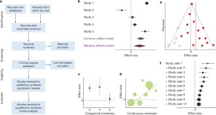
Persistent interaction patterns across social media platforms and over time

Michele Avalle, Niccolò Di Marco, … Walter Quattrociocchi

Life expectancy can increase by up to 10 years following sustained shifts towards healthier diets in the United Kingdom

Lars T. Fadnes, Carlos Celis-Morales, … John C. Mathers

Negativity drives online news consumption

Claire E. Robertson, Nicolas Pröllochs, … Stefan Feuerriegel

Jennions, M. D ., Lortie, C. J. & Koricheva, J. in The Handbook of Meta-analysis in Ecology and Evolution (eds Koricheva, J . et al.) Ch. 23 , 364–380 (Princeton Univ. Press, 2013)

Article   Google Scholar  

Roberts, P. D ., Stewart, G. B. & Pullin, A. S. Are review articles a reliable source of evidence to support conservation and environmental management? A comparison with medicine. Biol. Conserv. 132 , 409–423 (2006)

Bastian, H ., Glasziou, P . & Chalmers, I. Seventy-five trials and eleven systematic reviews a day: how will we ever keep up? PLoS Med. 7 , e1000326 (2010)

Article   PubMed   PubMed Central   Google Scholar  

Borman, G. D. & Grigg, J. A. in The Handbook of Research Synthesis and Meta-analysis 2nd edn (eds Cooper, H. M . et al.) 497–519 (Russell Sage Foundation, 2009)

Ioannidis, J. P. A. The mass production of redundant, misleading, and conflicted systematic reviews and meta-analyses. Milbank Q. 94 , 485–514 (2016)

Koricheva, J . & Gurevitch, J. Uses and misuses of meta-analysis in plant ecology. J. Ecol. 102 , 828–844 (2014)

Littell, J. H . & Shlonsky, A. Making sense of meta-analysis: a critique of “effectiveness of long-term psychodynamic psychotherapy”. Clin. Soc. Work J. 39 , 340–346 (2011)

Morrissey, M. B. Meta-analysis of magnitudes, differences and variation in evolutionary parameters. J. Evol. Biol. 29 , 1882–1904 (2016)

Article   CAS   PubMed   Google Scholar  

Whittaker, R. J. Meta-analyses and mega-mistakes: calling time on meta-analysis of the species richness-productivity relationship. Ecology 91 , 2522–2533 (2010)

Article   PubMed   Google Scholar  

Begley, C. G . & Ellis, L. M. Drug development: Raise standards for preclinical cancer research. Nature 483 , 531–533 (2012); clarification 485 , 41 (2012)

Article   CAS   ADS   PubMed   Google Scholar  

Hillebrand, H . & Cardinale, B. J. A critique for meta-analyses and the productivity-diversity relationship. Ecology 91 , 2545–2549 (2010)

Moher, D . et al. Preferred reporting items for systematic reviews and meta-analyses: the PRISMA statement. PLoS Med. 6 , e1000097 (2009). This paper provides a consensus regarding the reporting requirements for medical meta-analysis and has been highly influential in ensuring good reporting practice and standardizing language in evidence-based medicine, with further guidance for protocols, individual patient data meta-analyses and animal studies.

Moher, D . et al. Preferred reporting items for systematic review and meta-analysis protocols (PRISMA-P) 2015 statement. Syst. Rev. 4 , 1 (2015)

Nakagawa, S . & Santos, E. S. A. Methodological issues and advances in biological meta-analysis. Evol. Ecol. 26 , 1253–1274 (2012)

Nakagawa, S ., Noble, D. W. A ., Senior, A. M. & Lagisz, M. Meta-evaluation of meta-analysis: ten appraisal questions for biologists. BMC Biol. 15 , 18 (2017)

Hedges, L. & Olkin, I. Statistical Methods for Meta-analysis (Academic Press, 1985)

Viechtbauer, W. Conducting meta-analyses in R with the metafor package. J. Stat. Softw. 36 , 1–48 (2010)

Anzures-Cabrera, J . & Higgins, J. P. T. Graphical displays for meta-analysis: an overview with suggestions for practice. Res. Synth. Methods 1 , 66–80 (2010)

Egger, M ., Davey Smith, G ., Schneider, M. & Minder, C. Bias in meta-analysis detected by a simple, graphical test. Br. Med. J. 315 , 629–634 (1997)

Article   CAS   Google Scholar  

Duval, S . & Tweedie, R. Trim and fill: a simple funnel-plot-based method of testing and adjusting for publication bias in meta-analysis. Biometrics 56 , 455–463 (2000)

Article   CAS   MATH   PubMed   Google Scholar  

Leimu, R . & Koricheva, J. Cumulative meta-analysis: a new tool for detection of temporal trends and publication bias in ecology. Proc. R. Soc. Lond. B 271 , 1961–1966 (2004)

Higgins, J. P. T . & Green, S. (eds) Cochrane Handbook for Systematic Reviews of Interventions : Version 5.1.0 (Wiley, 2011). This large collaborative work provides definitive guidance for the production of systematic reviews in medicine and is of broad interest for methods development outside the medical field.

Lau, J ., Rothstein, H. R . & Stewart, G. B. in The Handbook of Meta-analysis in Ecology and Evolution (eds Koricheva, J . et al.) Ch. 25 , 407–419 (Princeton Univ. Press, 2013)

Lortie, C. J ., Stewart, G ., Rothstein, H. & Lau, J. How to critically read ecological meta-analyses. Res. Synth. Methods 6 , 124–133 (2015)

Murad, M. H . & Montori, V. M. Synthesizing evidence: shifting the focus from individual studies to the body of evidence. J. Am. Med. Assoc. 309 , 2217–2218 (2013)

Rasmussen, S. A ., Chu, S. Y ., Kim, S. Y ., Schmid, C. H . & Lau, J. Maternal obesity and risk of neural tube defects: a meta-analysis. Am. J. Obstet. Gynecol. 198 , 611–619 (2008)

Littell, J. H ., Campbell, M ., Green, S . & Toews, B. Multisystemic therapy for social, emotional, and behavioral problems in youth aged 10–17. Cochrane Database Syst. Rev. https://doi.org/10.1002/14651858.CD004797.pub4 (2005)

Schmidt, F. L. What do data really mean? Research findings, meta-analysis, and cumulative knowledge in psychology. Am. Psychol. 47 , 1173–1181 (1992)

Button, K. S . et al. Power failure: why small sample size undermines the reliability of neuroscience. Nat. Rev. Neurosci. 14 , 365–376 (2013); erratum 14 , 451 (2013)

Parker, T. H . et al. Transparency in ecology and evolution: real problems, real solutions. Trends Ecol. Evol. 31 , 711–719 (2016)

Stewart, G. Meta-analysis in applied ecology. Biol. Lett. 6 , 78–81 (2010)

Sutherland, W. J ., Pullin, A. S ., Dolman, P. M . & Knight, T. M. The need for evidence-based conservation. Trends Ecol. Evol. 19 , 305–308 (2004)

Lowry, E . et al. Biological invasions: a field synopsis, systematic review, and database of the literature. Ecol. Evol. 3 , 182–196 (2013)

Article   PubMed Central   Google Scholar  

Parmesan, C . & Yohe, G. A globally coherent fingerprint of climate change impacts across natural systems. Nature 421 , 37–42 (2003)

Jennions, M. D ., Lortie, C. J . & Koricheva, J. in The Handbook of Meta-analysis in Ecology and Evolution (eds Koricheva, J . et al.) Ch. 24 , 381–403 (Princeton Univ. Press, 2013)

Balvanera, P . et al. Quantifying the evidence for biodiversity effects on ecosystem functioning and services. Ecol. Lett. 9 , 1146–1156 (2006)

Cardinale, B. J . et al. Effects of biodiversity on the functioning of trophic groups and ecosystems. Nature 443 , 989–992 (2006)

Rey Benayas, J. M ., Newton, A. C ., Diaz, A. & Bullock, J. M. Enhancement of biodiversity and ecosystem services by ecological restoration: a meta-analysis. Science 325 , 1121–1124 (2009)

Article   ADS   PubMed   CAS   Google Scholar  

Leimu, R ., Mutikainen, P. I. A ., Koricheva, J. & Fischer, M. How general are positive relationships between plant population size, fitness and genetic variation? J. Ecol. 94 , 942–952 (2006)

Hillebrand, H. On the generality of the latitudinal diversity gradient. Am. Nat. 163 , 192–211 (2004)

Gurevitch, J. in The Handbook of Meta-analysis in Ecology and Evolution (eds Koricheva, J . et al.) Ch. 19 , 313–320 (Princeton Univ. Press, 2013)

Rustad, L . et al. A meta-analysis of the response of soil respiration, net nitrogen mineralization, and aboveground plant growth to experimental ecosystem warming. Oecologia 126 , 543–562 (2001)

Adams, D. C. Phylogenetic meta-analysis. Evolution 62 , 567–572 (2008)

Hadfield, J. D . & Nakagawa, S. General quantitative genetic methods for comparative biology: phylogenies, taxonomies and multi-trait models for continuous and categorical characters. J. Evol. Biol. 23 , 494–508 (2010)

Lajeunesse, M. J. Meta-analysis and the comparative phylogenetic method. Am. Nat. 174 , 369–381 (2009)

Rosenberg, M. S ., Adams, D. C . & Gurevitch, J. MetaWin: Statistical Software for Meta-Analysis with Resampling Tests Version 1 (Sinauer Associates, 1997)

Wallace, B. C . et al. OpenMEE: intuitive, open-source software for meta-analysis in ecology and evolutionary biology. Methods Ecol. Evol. 8 , 941–947 (2016)

Gurevitch, J ., Morrison, J. A . & Hedges, L. V. The interaction between competition and predation: a meta-analysis of field experiments. Am. Nat. 155 , 435–453 (2000)

Adams, D. C ., Gurevitch, J . & Rosenberg, M. S. Resampling tests for meta-analysis of ecological data. Ecology 78 , 1277–1283 (1997)

Gurevitch, J . & Hedges, L. V. Statistical issues in ecological meta-analyses. Ecology 80 , 1142–1149 (1999)

Schmid, C. H . & Mengersen, K. in The Handbook of Meta-analysis in Ecology and Evolution (eds Koricheva, J . et al.) Ch. 11 , 145–173 (Princeton Univ. Press, 2013)

Eysenck, H. J. Exercise in mega-silliness. Am. Psychol. 33 , 517 (1978)

Simberloff, D. Rejoinder to: Don’t calculate effect sizes; study ecological effects. Ecol. Lett. 9 , 921–922 (2006)

Cadotte, M. W ., Mehrkens, L. R . & Menge, D. N. L. Gauging the impact of meta-analysis on ecology. Evol. Ecol. 26 , 1153–1167 (2012)

Koricheva, J ., Jennions, M. D. & Lau, J. in The Handbook of Meta-analysis in Ecology and Evolution (eds Koricheva, J . et al.) Ch. 15 , 237–254 (Princeton Univ. Press, 2013)

Lau, J ., Ioannidis, J. P. A ., Terrin, N ., Schmid, C. H . & Olkin, I. The case of the misleading funnel plot. Br. Med. J. 333 , 597–600 (2006)

Vetter, D ., Rucker, G. & Storch, I. Meta-analysis: a need for well-defined usage in ecology and conservation biology. Ecosphere 4 , 1–24 (2013)

Mengersen, K ., Jennions, M. D. & Schmid, C. H. in The Handbook of Meta-analysis in Ecology and Evolution (eds Koricheva, J. et al.) Ch. 16 , 255–283 (Princeton Univ. Press, 2013)

Patsopoulos, N. A ., Analatos, A. A. & Ioannidis, J. P. A. Relative citation impact of various study designs in the health sciences. J. Am. Med. Assoc. 293 , 2362–2366 (2005)

Kueffer, C . et al. Fame, glory and neglect in meta-analyses. Trends Ecol. Evol. 26 , 493–494 (2011)

Cohnstaedt, L. W. & Poland, J. Review Articles: The black-market of scientific currency. Ann. Entomol. Soc. Am. 110 , 90 (2017)

Longo, D. L. & Drazen, J. M. Data sharing. N. Engl. J. Med. 374 , 276–277 (2016)

Gauch, H. G. Scientific Method in Practice (Cambridge Univ. Press, 2003)

Science Staff. Dealing with data: introduction. Challenges and opportunities. Science 331 , 692–693 (2011)

Nosek, B. A . et al. Promoting an open research culture. Science 348 , 1422–1425 (2015)

Article   CAS   ADS   PubMed   PubMed Central   Google Scholar  

Stewart, L. A . et al. Preferred reporting items for a systematic review and meta-analysis of individual participant data: the PRISMA-IPD statement. J. Am. Med. Assoc. 313 , 1657–1665 (2015)

Saldanha, I. J . et al. Evaluating Data Abstraction Assistant, a novel software application for data abstraction during systematic reviews: protocol for a randomized controlled trial. Syst. Rev. 5 , 196 (2016)

Tipton, E. & Pustejovsky, J. E. Small-sample adjustments for tests of moderators and model fit using robust variance estimation in meta-regression. J. Educ. Behav. Stat. 40 , 604–634 (2015)

Mengersen, K ., MacNeil, M. A . & Caley, M. J. The potential for meta-analysis to support decision analysis in ecology. Res. Synth. Methods 6 , 111–121 (2015)

Ashby, D. Bayesian statistics in medicine: a 25 year review. Stat. Med. 25 , 3589–3631 (2006)

Article   MathSciNet   PubMed   Google Scholar  

Senior, A. M . et al. Heterogeneity in ecological and evolutionary meta-analyses: its magnitude and implications. Ecology 97 , 3293–3299 (2016)

McAuley, L ., Pham, B ., Tugwell, P . & Moher, D. Does the inclusion of grey literature influence estimates of intervention effectiveness reported in meta-analyses? Lancet 356 , 1228–1231 (2000)

Koricheva, J ., Gurevitch, J . & Mengersen, K. (eds) The Handbook of Meta-Analysis in Ecology and Evolution (Princeton Univ. Press, 2013) This book provides the first comprehensive guide to undertaking meta-analyses in ecology and evolution and is also relevant to other fields where heterogeneity is expected, incorporating explicit consideration of the different approaches used in different domains.

Lumley, T. Network meta-analysis for indirect treatment comparisons. Stat. Med. 21 , 2313–2324 (2002)

Zarin, W . et al. Characteristics and knowledge synthesis approach for 456 network meta-analyses: a scoping review. BMC Med. 15 , 3 (2017)

Elliott, J. H . et al. Living systematic reviews: an emerging opportunity to narrow the evidence-practice gap. PLoS Med. 11 , e1001603 (2014)

Vandvik, P. O ., Brignardello-Petersen, R . & Guyatt, G. H. Living cumulative network meta-analysis to reduce waste in research: a paradigmatic shift for systematic reviews? BMC Med. 14 , 59 (2016)

Jarvinen, A. A meta-analytic study of the effects of female age on laying date and clutch size in the Great Tit Parus major and the Pied Flycatcher Ficedula hypoleuca . Ibis 133 , 62–67 (1991)

Arnqvist, G. & Wooster, D. Meta-analysis: synthesizing research findings in ecology and evolution. Trends Ecol. Evol. 10 , 236–240 (1995)

Hedges, L. V ., Gurevitch, J . & Curtis, P. S. The meta-analysis of response ratios in experimental ecology. Ecology 80 , 1150–1156 (1999)

Gurevitch, J ., Curtis, P. S. & Jones, M. H. Meta-analysis in ecology. Adv. Ecol. Res 32 , 199–247 (2001)

Lajeunesse, M. J. phyloMeta: a program for phylogenetic comparative analyses with meta-analysis. Bioinformatics 27 , 2603–2604 (2011)

CAS   PubMed   Google Scholar  

Pearson, K. Report on certain enteric fever inoculation statistics. Br. Med. J. 2 , 1243–1246 (1904)

Fisher, R. A. Statistical Methods for Research Workers (Oliver and Boyd, 1925)

Yates, F. & Cochran, W. G. The analysis of groups of experiments. J. Agric. Sci. 28 , 556–580 (1938)

Cochran, W. G. The combination of estimates from different experiments. Biometrics 10 , 101–129 (1954)

Smith, M. L . & Glass, G. V. Meta-analysis of psychotherapy outcome studies. Am. Psychol. 32 , 752–760 (1977)

Glass, G. V. Meta-analysis at middle age: a personal history. Res. Synth. Methods 6 , 221–231 (2015)

Cooper, H. M ., Hedges, L. V . & Valentine, J. C. (eds) The Handbook of Research Synthesis and Meta-analysis 2nd edn (Russell Sage Foundation, 2009). This book is an important compilation that builds on the ground-breaking first edition to set the standard for best practice in meta-analysis, primarily in the social sciences but with applications to medicine and other fields.

Rosenthal, R. Meta-analytic Procedures for Social Research (Sage, 1991)

Hunter, J. E ., Schmidt, F. L. & Jackson, G. B. Meta-analysis: Cumulating Research Findings Across Studies (Sage, 1982)

Gurevitch, J ., Morrow, L. L ., Wallace, A . & Walsh, J. S. A meta-analysis of competition in field experiments. Am. Nat. 140 , 539–572 (1992). This influential early ecological meta-analysis reports multiple experimental outcomes on a longstanding and controversial topic that introduced a wide range of ecologists to research synthesis methods.

O’Rourke, K. An historical perspective on meta-analysis: dealing quantitatively with varying study results. J. R. Soc. Med. 100 , 579–582 (2007)

Shadish, W. R . & Lecy, J. D. The meta-analytic big bang. Res. Synth. Methods 6 , 246–264 (2015)

Glass, G. V. Primary, secondary, and meta-analysis of research. Educ. Res. 5 , 3–8 (1976)

DerSimonian, R . & Laird, N. Meta-analysis in clinical trials. Control. Clin. Trials 7 , 177–188 (1986)

Lipsey, M. W . & Wilson, D. B. The efficacy of psychological, educational, and behavioral treatment. Confirmation from meta-analysis. Am. Psychol. 48 , 1181–1209 (1993)

Chalmers, I. & Altman, D. G. Systematic Reviews (BMJ Publishing Group, 1995)

Moher, D . et al. Improving the quality of reports of meta-analyses of randomised controlled trials: the QUOROM statement. Quality of reporting of meta-analyses. Lancet 354 , 1896–1900 (1999)

Higgins, J. P. & Thompson, S. G. Quantifying heterogeneity in a meta-analysis. Stat. Med. 21 , 1539–1558 (2002)

Download references

Acknowledgements

We dedicate this Review to the memory of Ingram Olkin and William Shadish, founding members of the Society for Research Synthesis Methodology who made tremendous contributions to the development of meta-analysis and research synthesis and to the supervision of generations of students. We thank L. Lagisz for help in preparing the figures. We are grateful to the Center for Open Science and the Laura and John Arnold Foundation for hosting and funding a workshop, which was the origination of this article. S.N. is supported by Australian Research Council Future Fellowship (FT130100268). J.G. acknowledges funding from the US National Science Foundation (ABI 1262402).

Author information

Authors and affiliations.

Department of Ecology and Evolution, Stony Brook University, Stony Brook, 11794-5245, New York, USA

Jessica Gurevitch

School of Biological Sciences, Royal Holloway University of London, Egham, TW20 0EX, Surrey, UK

Julia Koricheva

Evolution and Ecology Research Centre and School of Biological, Earth and Environmental Sciences, University of New South Wales, Sydney, 2052, New South Wales, Australia

Shinichi Nakagawa

Diabetes and Metabolism Division, Garvan Institute of Medical Research, 384 Victoria Street, Darlinghurst, Sydney, 2010, New South Wales, Australia

School of Natural and Environmental Sciences, Newcastle University, Newcastle upon Tyne, NE1 7RU, UK

Gavin Stewart

You can also search for this author in PubMed   Google Scholar

Contributions

All authors contributed equally in designing the study and writing the manuscript, and so are listed alphabetically.

Corresponding authors

Correspondence to Jessica Gurevitch , Julia Koricheva , Shinichi Nakagawa or Gavin Stewart .

Ethics declarations

Competing interests.

The authors declare no competing financial interests.

Additional information

Reviewer Information Nature thanks D. Altman, M. Lajeunesse, D. Moher and G. Romero for their contribution to the peer review of this work.

Publisher's note: Springer Nature remains neutral with regard to jurisdictional claims in published maps and institutional affiliations.

PowerPoint slides

Powerpoint slide for fig. 1, rights and permissions.

Reprints and permissions

About this article

Cite this article.

Gurevitch, J., Koricheva, J., Nakagawa, S. et al. Meta-analysis and the science of research synthesis. Nature 555 , 175–182 (2018). https://doi.org/10.1038/nature25753

Download citation

Received : 04 March 2017

Accepted : 12 January 2018

Published : 08 March 2018

Issue Date : 08 March 2018

DOI : https://doi.org/10.1038/nature25753

Share this article

Anyone you share the following link with will be able to read this content:

Sorry, a shareable link is not currently available for this article.

Provided by the Springer Nature SharedIt content-sharing initiative

This article is cited by

Investigate the relationship between the retraction reasons and the quality of methodology in non-cochrane retracted systematic reviews: a systematic review.

• Azita Shahraki-Mohammadi
• Leila Keikha
• Razieh Zahedi

Systematic Reviews (2024)

Systematic review of the uncertainty of coral reef futures under climate change

• Shannon G. Klein
• Cassandra Roch
• Carlos M. Duarte

Nature Communications (2024)

Meta-analysis reveals weak associations between reef fishes and corals

• Pooventhran Muruga
• Alexandre C. Siqueira
• David R. Bellwood

Nature Ecology & Evolution (2024)

Farming practices to enhance biodiversity across biomes: a systematic review

• Felipe Cozim-Melges
• Raimon Ripoll-Bosch
• Hannah H. E. van Zanten

npj Biodiversity (2024)

Bacillus species as tools for biocontrol of plant diseases: A meta-analysis of twenty-two years of research, 2000–2021

• Cleyson Pantoja Serrão
• Jean Carlo Gonçalves Ortega
• Cláudia Regina Batista de Souza

World Journal of Microbiology and Biotechnology (2024)

By submitting a comment you agree to abide by our Terms and Community Guidelines . If you find something abusive or that does not comply with our terms or guidelines please flag it as inappropriate.

Quick links

• Explore articles by subject
• Guide to authors
• Editorial policies

Sign up for the Nature Briefing newsletter — what matters in science, free to your inbox daily.

Jump to navigation

Cochrane Training

Chapter 10: analysing data and undertaking meta-analyses.

Jonathan J Deeks, Julian PT Higgins, Douglas G Altman; on behalf of the Cochrane Statistical Methods Group

Key Points:

• Meta-analysis is the statistical combination of results from two or more separate studies.
• Potential advantages of meta-analyses include an improvement in precision, the ability to answer questions not posed by individual studies, and the opportunity to settle controversies arising from conflicting claims. However, they also have the potential to mislead seriously, particularly if specific study designs, within-study biases, variation across studies, and reporting biases are not carefully considered.
• It is important to be familiar with the type of data (e.g. dichotomous, continuous) that result from measurement of an outcome in an individual study, and to choose suitable effect measures for comparing intervention groups.
• Most meta-analysis methods are variations on a weighted average of the effect estimates from the different studies.
• Studies with no events contribute no information about the risk ratio or odds ratio. For rare events, the Peto method has been observed to be less biased and more powerful than other methods.
• Variation across studies (heterogeneity) must be considered, although most Cochrane Reviews do not have enough studies to allow for the reliable investigation of its causes. Random-effects meta-analyses allow for heterogeneity by assuming that underlying effects follow a normal distribution, but they must be interpreted carefully. Prediction intervals from random-effects meta-analyses are a useful device for presenting the extent of between-study variation.
• Many judgements are required in the process of preparing a meta-analysis. Sensitivity analyses should be used to examine whether overall findings are robust to potentially influential decisions.

Cite this chapter as: Deeks JJ, Higgins JPT, Altman DG (editors). Chapter 10: Analysing data and undertaking meta-analyses. In: Higgins JPT, Thomas J, Chandler J, Cumpston M, Li T, Page MJ, Welch VA (editors). Cochrane Handbook for Systematic Reviews of Interventions version 6.4 (updated August  2023). Cochrane, 2023. Available from www.training.cochrane.org/handbook .

10.1 Do not start here!

It can be tempting to jump prematurely into a statistical analysis when undertaking a systematic review. The production of a diamond at the bottom of a plot is an exciting moment for many authors, but results of meta-analyses can be very misleading if suitable attention has not been given to formulating the review question; specifying eligibility criteria; identifying and selecting studies; collecting appropriate data; considering risk of bias; planning intervention comparisons; and deciding what data would be meaningful to analyse. Review authors should consult the chapters that precede this one before a meta-analysis is undertaken.

10.2 Introduction to meta-analysis

An important step in a systematic review is the thoughtful consideration of whether it is appropriate to combine the numerical results of all, or perhaps some, of the studies. Such a meta-analysis yields an overall statistic (together with its confidence interval) that summarizes the effectiveness of an experimental intervention compared with a comparator intervention. Potential advantages of meta-analyses include the following:

• T o improve precision . Many studies are too small to provide convincing evidence about intervention effects in isolation. Estimation is usually improved when it is based on more information.
• To answer questions not posed by the individual studies . Primary studies often involve a specific type of participant and explicitly defined interventions. A selection of studies in which these characteristics differ can allow investigation of the consistency of effect across a wider range of populations and interventions. It may also, if relevant, allow reasons for differences in effect estimates to be investigated.
• To settle controversies arising from apparently conflicting studies or to generate new hypotheses . Statistical synthesis of findings allows the degree of conflict to be formally assessed, and reasons for different results to be explored and quantified.

Of course, the use of statistical synthesis methods does not guarantee that the results of a review are valid, any more than it does for a primary study. Moreover, like any tool, statistical methods can be misused.

This chapter describes the principles and methods used to carry out a meta-analysis for a comparison of two interventions for the main types of data encountered. The use of network meta-analysis to compare more than two interventions is addressed in Chapter 11 . Formulae for most of the methods described are provided in the RevMan Web Knowledge Base under Statistical Algorithms and calculations used in Review Manager (documentation.cochrane.org/revman-kb/statistical-methods-210600101.html), and a longer discussion of many of the issues is available ( Deeks et al 2001 ).

10.2.1 Principles of meta-analysis

The commonly used methods for meta-analysis follow the following basic principles:

• Meta-analysis is typically a two-stage process. In the first stage, a summary statistic is calculated for each study, to describe the observed intervention effect in the same way for every study. For example, the summary statistic may be a risk ratio if the data are dichotomous, or a difference between means if the data are continuous (see Chapter 6 ).

• The combination of intervention effect estimates across studies may optionally incorporate an assumption that the studies are not all estimating the same intervention effect, but estimate intervention effects that follow a distribution across studies. This is the basis of a random-effects meta-analysis (see Section 10.10.4 ). Alternatively, if it is assumed that each study is estimating exactly the same quantity, then a fixed-effect meta-analysis is performed.
• The standard error of the summary intervention effect can be used to derive a confidence interval, which communicates the precision (or uncertainty) of the summary estimate; and to derive a P value, which communicates the strength of the evidence against the null hypothesis of no intervention effect.
• As well as yielding a summary quantification of the intervention effect, all methods of meta-analysis can incorporate an assessment of whether the variation among the results of the separate studies is compatible with random variation, or whether it is large enough to indicate inconsistency of intervention effects across studies (see Section 10.10 ).
• The problem of missing data is one of the numerous practical considerations that must be thought through when undertaking a meta-analysis. In particular, review authors should consider the implications of missing outcome data from individual participants (due to losses to follow-up or exclusions from analysis) (see Section 10.12 ).

Meta-analyses are usually illustrated using a forest plot . An example appears in Figure 10.2.a . A forest plot displays effect estimates and confidence intervals for both individual studies and meta-analyses (Lewis and Clarke 2001). Each study is represented by a block at the point estimate of intervention effect with a horizontal line extending either side of the block. The area of the block indicates the weight assigned to that study in the meta-analysis while the horizontal line depicts the confidence interval (usually with a 95% level of confidence). The area of the block and the confidence interval convey similar information, but both make different contributions to the graphic. The confidence interval depicts the range of intervention effects compatible with the study’s result. The size of the block draws the eye towards the studies with larger weight (usually those with narrower confidence intervals), which dominate the calculation of the summary result, presented as a diamond at the bottom.

Figure 10.2.a Example of a forest plot from a review of interventions to promote ownership of smoke alarms (DiGuiseppi and Higgins 2001). Reproduced with permission of John Wiley & Sons

10.3 A generic inverse-variance approach to meta-analysis

A very common and simple version of the meta-analysis procedure is commonly referred to as the inverse-variance method . This approach is implemented in its most basic form in RevMan, and is used behind the scenes in many meta-analyses of both dichotomous and continuous data.

The inverse-variance method is so named because the weight given to each study is chosen to be the inverse of the variance of the effect estimate (i.e. 1 over the square of its standard error). Thus, larger studies, which have smaller standard errors, are given more weight than smaller studies, which have larger standard errors. This choice of weights minimizes the imprecision (uncertainty) of the pooled effect estimate.

10.3.1 Fixed-effect method for meta-analysis

A fixed-effect meta-analysis using the inverse-variance method calculates a weighted average as:

where Y i is the intervention effect estimated in the i th study, SE i is the standard error of that estimate, and the summation is across all studies. The basic data required for the analysis are therefore an estimate of the intervention effect and its standard error from each study. A fixed-effect meta-analysis is valid under an assumption that all effect estimates are estimating the same underlying intervention effect, which is referred to variously as a ‘fixed-effect’ assumption, a ‘common-effect’ assumption or an ‘equal-effects’ assumption. However, the result of the meta-analysis can be interpreted without making such an assumption (Rice et al 2018).

10.3.2 Random-effects methods for meta-analysis

A variation on the inverse-variance method is to incorporate an assumption that the different studies are estimating different, yet related, intervention effects (Higgins et al 2009). This produces a random-effects meta-analysis, and the simplest version is known as the DerSimonian and Laird method (DerSimonian and Laird 1986). Random-effects meta-analysis is discussed in detail in Section 10.10.4 .

10.3.3 Performing inverse-variance meta-analyses

Most meta-analysis programs perform inverse-variance meta-analyses. Usually the user provides summary data from each intervention arm of each study, such as a 2×2 table when the outcome is dichotomous (see Chapter 6, Section 6.4 ), or means, standard deviations and sample sizes for each group when the outcome is continuous (see Chapter 6, Section 6.5 ). This avoids the need for the author to calculate effect estimates, and allows the use of methods targeted specifically at different types of data (see Sections 10.4 and 10.5 ).

When the data are conveniently available as summary statistics from each intervention group, the inverse-variance method can be implemented directly. For example, estimates and their standard errors may be entered directly into RevMan under the ‘Generic inverse variance’ outcome type. For ratio measures of intervention effect, the data must be entered into RevMan as natural logarithms (for example, as a log odds ratio and the standard error of the log odds ratio). However, it is straightforward to instruct the software to display results on the original (e.g. odds ratio) scale. It is possible to supplement or replace this with a column providing the sample sizes in the two groups. Note that the ability to enter estimates and standard errors creates a high degree of flexibility in meta-analysis. It facilitates the analysis of properly analysed crossover trials, cluster-randomized trials and non-randomized trials (see Chapter 23 ), as well as outcome data that are ordinal, time-to-event or rates (see Chapter 6 ).

10.4 Meta-analysis of dichotomous outcomes

There are four widely used methods of meta-analysis for dichotomous outcomes, three fixed-effect methods (Mantel-Haenszel, Peto and inverse variance) and one random-effects method (DerSimonian and Laird inverse variance). All of these methods are available as analysis options in RevMan. The Peto method can only combine odds ratios, whilst the other three methods can combine odds ratios, risk ratios or risk differences. Formulae for all of the meta-analysis methods are available elsewhere (Deeks et al 2001).

Note that having no events in one group (sometimes referred to as ‘zero cells’) causes problems with computation of estimates and standard errors with some methods: see Section 10.4.4 .

10.4.1 Mantel-Haenszel methods

When data are sparse, either in terms of event risks being low or study size being small, the estimates of the standard errors of the effect estimates that are used in the inverse-variance methods may be poor. Mantel-Haenszel methods are fixed-effect meta-analysis methods using a different weighting scheme that depends on which effect measure (e.g. risk ratio, odds ratio, risk difference) is being used (Mantel and Haenszel 1959, Greenland and Robins 1985). They have been shown to have better statistical properties when there are few events. As this is a common situation in Cochrane Reviews, the Mantel-Haenszel method is generally preferable to the inverse variance method in fixed-effect meta-analyses. In other situations the two methods give similar estimates.

10.4.2 Peto odds ratio method

Peto’s method can only be used to combine odds ratios (Yusuf et al 1985). It uses an inverse-variance approach, but uses an approximate method of estimating the log odds ratio, and uses different weights. An alternative way of viewing the Peto method is as a sum of ‘O – E’ statistics. Here, O is the observed number of events and E is an expected number of events in the experimental intervention group of each study under the null hypothesis of no intervention effect.

The approximation used in the computation of the log odds ratio works well when intervention effects are small (odds ratios are close to 1), events are not particularly common and the studies have similar numbers in experimental and comparator groups. In other situations it has been shown to give biased answers. As these criteria are not always fulfilled, Peto’s method is not recommended as a default approach for meta-analysis.

Corrections for zero cell counts are not necessary when using Peto’s method. Perhaps for this reason, this method performs well when events are very rare (Bradburn et al 2007); see Section 10.4.4.1 . Also, Peto’s method can be used to combine studies with dichotomous outcome data with studies using time-to-event analyses where log-rank tests have been used (see Section 10.9 ).

10.4.3 Which effect measure for dichotomous outcomes?

Effect measures for dichotomous data are described in Chapter 6, Section 6.4.1 . The effect of an intervention can be expressed as either a relative or an absolute effect. The risk ratio (relative risk) and odds ratio are relative measures, while the risk difference and number needed to treat for an additional beneficial outcome are absolute measures. A further complication is that there are, in fact, two risk ratios. We can calculate the risk ratio of an event occurring or the risk ratio of no event occurring. These give different summary results in a meta-analysis, sometimes dramatically so.

The selection of a summary statistic for use in meta-analysis depends on balancing three criteria (Deeks 2002). First, we desire a summary statistic that gives values that are similar for all the studies in the meta-analysis and subdivisions of the population to which the interventions will be applied. The more consistent the summary statistic, the greater is the justification for expressing the intervention effect as a single summary number. Second, the summary statistic must have the mathematical properties required to perform a valid meta-analysis. Third, the summary statistic would ideally be easily understood and applied by those using the review. The summary intervention effect should be presented in a way that helps readers to interpret and apply the results appropriately. Among effect measures for dichotomous data, no single measure is uniformly best, so the choice inevitably involves a compromise.

Consistency Empirical evidence suggests that relative effect measures are, on average, more consistent than absolute measures (Engels et al 2000, Deeks 2002, Rücker et al 2009). For this reason, it is wise to avoid performing meta-analyses of risk differences, unless there is a clear reason to suspect that risk differences will be consistent in a particular clinical situation. On average there is little difference between the odds ratio and risk ratio in terms of consistency (Deeks 2002). When the study aims to reduce the incidence of an adverse event, there is empirical evidence that risk ratios of the adverse event are more consistent than risk ratios of the non-event (Deeks 2002). Selecting an effect measure based on what is the most consistent in a particular situation is not a generally recommended strategy, since it may lead to a selection that spuriously maximizes the precision of a meta-analysis estimate.

Mathematical properties The most important mathematical criterion is the availability of a reliable variance estimate. The number needed to treat for an additional beneficial outcome does not have a simple variance estimator and cannot easily be used directly in meta-analysis, although it can be computed from the meta-analysis result afterwards (see Chapter 15, Section 15.4.2 ). There is no consensus regarding the importance of two other often-cited mathematical properties: the fact that the behaviour of the odds ratio and the risk difference do not rely on which of the two outcome states is coded as the event, and the odds ratio being the only statistic which is unbounded (see Chapter 6, Section 6.4.1 ).

Ease of interpretation The odds ratio is the hardest summary statistic to understand and to apply in practice, and many practising clinicians report difficulties in using them. There are many published examples where authors have misinterpreted odds ratios from meta-analyses as risk ratios. Although odds ratios can be re-expressed for interpretation (as discussed here), there must be some concern that routine presentation of the results of systematic reviews as odds ratios will lead to frequent over-estimation of the benefits and harms of interventions when the results are applied in clinical practice. Absolute measures of effect are thought to be more easily interpreted by clinicians than relative effects (Sinclair and Bracken 1994), and allow trade-offs to be made between likely benefits and likely harms of interventions. However, they are less likely to be generalizable.

It is generally recommended that meta-analyses are undertaken using risk ratios (taking care to make a sensible choice over which category of outcome is classified as the event) or odds ratios. This is because it seems important to avoid using summary statistics for which there is empirical evidence that they are unlikely to give consistent estimates of intervention effects (the risk difference), and it is impossible to use statistics for which meta-analysis cannot be performed (the number needed to treat for an additional beneficial outcome). It may be wise to plan to undertake a sensitivity analysis to investigate whether choice of summary statistic (and selection of the event category) is critical to the conclusions of the meta-analysis (see Section 10.14 ).

It is often sensible to use one statistic for meta-analysis and to re-express the results using a second, more easily interpretable statistic. For example, often meta-analysis may be best performed using relative effect measures (risk ratios or odds ratios) and the results re-expressed using absolute effect measures (risk differences or numbers needed to treat for an additional beneficial outcome – see Chapter 15, Section 15.4 . This is one of the key motivations for ‘Summary of findings’ tables in Cochrane Reviews: see Chapter 14 ). If odds ratios are used for meta-analysis they can also be re-expressed as risk ratios (see Chapter 15, Section 15.4 ). In all cases the same formulae can be used to convert upper and lower confidence limits. However, all of these transformations require specification of a value of baseline risk that indicates the likely risk of the outcome in the ‘control’ population to which the experimental intervention will be applied. Where the chosen value for this assumed comparator group risk is close to the typical observed comparator group risks across the studies, similar estimates of absolute effect will be obtained regardless of whether odds ratios or risk ratios are used for meta-analysis. Where the assumed comparator risk differs from the typical observed comparator group risk, the predictions of absolute benefit will differ according to which summary statistic was used for meta-analysis.

10.4.4 Meta-analysis of rare events

For rare outcomes, meta-analysis may be the only way to obtain reliable evidence of the effects of healthcare interventions. Individual studies are usually under-powered to detect differences in rare outcomes, but a meta-analysis of many studies may have adequate power to investigate whether interventions do have an impact on the incidence of the rare event. However, many methods of meta-analysis are based on large sample approximations, and are unsuitable when events are rare. Thus authors must take care when selecting a method of meta-analysis (Efthimiou 2018).

There is no single risk at which events are classified as ‘rare’. Certainly risks of 1 in 1000 constitute rare events, and many would classify risks of 1 in 100 the same way. However, the performance of methods when risks are as high as 1 in 10 may also be affected by the issues discussed in this section. What is typical is that a high proportion of the studies in the meta-analysis observe no events in one or more study arms.

10.4.4.1 Studies with no events in one or more arms

Computational problems can occur when no events are observed in one or both groups in an individual study. Inverse variance meta-analytical methods involve computing an intervention effect estimate and its standard error for each study. For studies where no events were observed in one or both arms, these computations often involve dividing by a zero count, which yields a computational error. Most meta-analytical software routines (including those in RevMan) automatically check for problematic zero counts, and add a fixed value (typically 0.5) to all cells of a 2×2 table where the problems occur. The Mantel-Haenszel methods require zero-cell corrections only if the same cell is zero in all the included studies, and hence need to use the correction less often. However, in many software applications the same correction rules are applied for Mantel-Haenszel methods as for the inverse-variance methods. Odds ratio and risk ratio methods require zero cell corrections more often than difference methods, except for the Peto odds ratio method, which encounters computation problems only in the extreme situation of no events occurring in all arms of all studies.

Whilst the fixed correction meets the objective of avoiding computational errors, it usually has the undesirable effect of biasing study estimates towards no difference and over-estimating variances of study estimates (consequently down-weighting inappropriately their contribution to the meta-analysis). Where the sizes of the study arms are unequal (which occurs more commonly in non-randomized studies than randomized trials), they will introduce a directional bias in the treatment effect. Alternative non-fixed zero-cell corrections have been explored by Sweeting and colleagues, including a correction proportional to the reciprocal of the size of the contrasting study arm, which they found preferable to the fixed 0.5 correction when arm sizes were not balanced (Sweeting et al 2004).

10.4.4.2 Studies with no events in either arm

The standard practice in meta-analysis of odds ratios and risk ratios is to exclude studies from the meta-analysis where there are no events in both arms. This is because such studies do not provide any indication of either the direction or magnitude of the relative treatment effect. Whilst it may be clear that events are very rare on both the experimental intervention and the comparator intervention, no information is provided as to which group is likely to have the higher risk, or on whether the risks are of the same or different orders of magnitude (when risks are very low, they are compatible with very large or very small ratios). Whilst one might be tempted to infer that the risk would be lowest in the group with the larger sample size (as the upper limit of the confidence interval would be lower), this is not justified as the sample size allocation was determined by the study investigators and is not a measure of the incidence of the event.

Risk difference methods superficially appear to have an advantage over odds ratio methods in that the risk difference is defined (as zero) when no events occur in either arm. Such studies are therefore included in the estimation process. Bradburn and colleagues undertook simulation studies which revealed that all risk difference methods yield confidence intervals that are too wide when events are rare, and have associated poor statistical power, which make them unsuitable for meta-analysis of rare events (Bradburn et al 2007). This is especially relevant when outcomes that focus on treatment safety are being studied, as the ability to identify correctly (or attempt to refute) serious adverse events is a key issue in drug development.

It is likely that outcomes for which no events occur in either arm may not be mentioned in reports of many randomized trials, precluding their inclusion in a meta-analysis. It is unclear, though, when working with published results, whether failure to mention a particular adverse event means there were no such events, or simply that such events were not included as a measured endpoint. Whilst the results of risk difference meta-analyses will be affected by non-reporting of outcomes with no events, odds and risk ratio based methods naturally exclude these data whether or not they are published, and are therefore unaffected.

10.4.4.3 Validity of methods of meta-analysis for rare events

Simulation studies have revealed that many meta-analytical methods can give misleading results for rare events, which is unsurprising given their reliance on asymptotic statistical theory. Their performance has been judged suboptimal either through results being biased, confidence intervals being inappropriately wide, or statistical power being too low to detect substantial differences.

In the following we consider the choice of statistical method for meta-analyses of odds ratios. Appropriate choices appear to depend on the comparator group risk, the likely size of the treatment effect and consideration of balance in the numbers of experimental and comparator participants in the constituent studies. We are not aware of research that has evaluated risk ratio measures directly, but their performance is likely to be very similar to corresponding odds ratio measurements. When events are rare, estimates of odds and risks are near identical, and results of both can be interpreted as ratios of probabilities.

Bradburn and colleagues found that many of the most commonly used meta-analytical methods were biased when events were rare (Bradburn et al 2007). The bias was greatest in inverse variance and DerSimonian and Laird odds ratio and risk difference methods, and the Mantel-Haenszel odds ratio method using a 0.5 zero-cell correction. As already noted, risk difference meta-analytical methods tended to show conservative confidence interval coverage and low statistical power when risks of events were low.

At event rates below 1% the Peto one-step odds ratio method was found to be the least biased and most powerful method, and provided the best confidence interval coverage, provided there was no substantial imbalance between treatment and comparator group sizes within studies, and treatment effects were not exceptionally large. This finding was consistently observed across three different meta-analytical scenarios, and was also observed by Sweeting and colleagues (Sweeting et al 2004).

This finding was noted despite the method producing only an approximation to the odds ratio. For very large effects (e.g. risk ratio=0.2) when the approximation is known to be poor, treatment effects were under-estimated, but the Peto method still had the best performance of all the methods considered for event risks of 1 in 1000, and the bias was never more than 6% of the comparator group risk.

In other circumstances (i.e. event risks above 1%, very large effects at event risks around 1%, and meta-analyses where many studies were substantially imbalanced) the best performing methods were the Mantel-Haenszel odds ratio without zero-cell corrections, logistic regression and an exact method. None of these methods is available in RevMan.

Methods that should be avoided with rare events are the inverse-variance methods (including the DerSimonian and Laird random-effects method) (Efthimiou 2018). These directly incorporate the study’s variance in the estimation of its contribution to the meta-analysis, but these are usually based on a large-sample variance approximation, which was not intended for use with rare events. We would suggest that incorporation of heterogeneity into an estimate of a treatment effect should be a secondary consideration when attempting to produce estimates of effects from sparse data – the primary concern is to discern whether there is any signal of an effect in the data.

10.5 Meta-analysis of continuous outcomes

An important assumption underlying standard methods for meta-analysis of continuous data is that the outcomes have a normal distribution in each intervention arm in each study. This assumption may not always be met, although it is unimportant in very large studies. It is useful to consider the possibility of skewed data (see Section 10.5.3 ).

10.5.1 Which effect measure for continuous outcomes?

The two summary statistics commonly used for meta-analysis of continuous data are the mean difference (MD) and the standardized mean difference (SMD). Other options are available, such as the ratio of means (see Chapter 6, Section 6.5.1 ). Selection of summary statistics for continuous data is principally determined by whether studies all report the outcome using the same scale (when the mean difference can be used) or using different scales (when the standardized mean difference is usually used). The ratio of means can be used in either situation, but is appropriate only when outcome measurements are strictly greater than zero. Further considerations in deciding on an effect measure that will facilitate interpretation of the findings appears in Chapter 15, Section 15.5 .

The different roles played in MD and SMD approaches by the standard deviations (SDs) of outcomes observed in the two groups should be understood.

For the mean difference approach, the SDs are used together with the sample sizes to compute the weight given to each study. Studies with small SDs are given relatively higher weight whilst studies with larger SDs are given relatively smaller weights. This is appropriate if variation in SDs between studies reflects differences in the reliability of outcome measurements, but is probably not appropriate if the differences in SD reflect real differences in the variability of outcomes in the study populations.

For the standardized mean difference approach, the SDs are used to standardize the mean differences to a single scale, as well as in the computation of study weights. Thus, studies with small SDs lead to relatively higher estimates of SMD, whilst studies with larger SDs lead to relatively smaller estimates of SMD. For this to be appropriate, it must be assumed that between-study variation in SDs reflects only differences in measurement scales and not differences in the reliability of outcome measures or variability among study populations, as discussed in Chapter 6, Section 6.5.1.2 .

These assumptions of the methods should be borne in mind when unexpected variation of SDs is observed across studies.

10.5.2 Meta-analysis of change scores

In some circumstances an analysis based on changes from baseline will be more efficient and powerful than comparison of post-intervention values, as it removes a component of between-person variability from the analysis. However, calculation of a change score requires measurement of the outcome twice and in practice may be less efficient for outcomes that are unstable or difficult to measure precisely, where the measurement error may be larger than true between-person baseline variability. Change-from-baseline outcomes may also be preferred if they have a less skewed distribution than post-intervention measurement outcomes. Although sometimes used as a device to ‘correct’ for unlucky randomization, this practice is not recommended.

The preferred statistical approach to accounting for baseline measurements of the outcome variable is to include the baseline outcome measurements as a covariate in a regression model or analysis of covariance (ANCOVA). These analyses produce an ‘adjusted’ estimate of the intervention effect together with its standard error. These analyses are the least frequently encountered, but as they give the most precise and least biased estimates of intervention effects they should be included in the analysis when they are available. However, they can only be included in a meta-analysis using the generic inverse-variance method, since means and SDs are not available for each intervention group separately.

In practice an author is likely to discover that the studies included in a review include a mixture of change-from-baseline and post-intervention value scores. However, mixing of outcomes is not a problem when it comes to meta-analysis of MDs. There is no statistical reason why studies with change-from-baseline outcomes should not be combined in a meta-analysis with studies with post-intervention measurement outcomes when using the (unstandardized) MD method. In a randomized study, MD based on changes from baseline can usually be assumed to be addressing exactly the same underlying intervention effects as analyses based on post-intervention measurements. That is to say, the difference in mean post-intervention values will on average be the same as the difference in mean change scores. If the use of change scores does increase precision, appropriately, the studies presenting change scores will be given higher weights in the analysis than they would have received if post-intervention values had been used, as they will have smaller SDs.

When combining the data on the MD scale, authors must be careful to use the appropriate means and SDs (either of post-intervention measurements or of changes from baseline) for each study. Since the mean values and SDs for the two types of outcome may differ substantially, it may be advisable to place them in separate subgroups to avoid confusion for the reader, but the results of the subgroups can legitimately be pooled together.

In contrast, post-intervention value and change scores should not in principle be combined using standard meta-analysis approaches when the effect measure is an SMD. This is because the SDs used in the standardization reflect different things. The SD when standardizing post-intervention values reflects between-person variability at a single point in time. The SD when standardizing change scores reflects variation in between-person changes over time, so will depend on both within-person and between-person variability; within-person variability in turn is likely to depend on the length of time between measurements. Nevertheless, an empirical study of 21 meta-analyses in osteoarthritis did not find a difference between combined SMDs based on post-intervention values and combined SMDs based on change scores (da Costa et al 2013). One option is to standardize SMDs using post-intervention SDs rather than change score SDs. This would lead to valid synthesis of the two approaches, but we are not aware that an appropriate standard error for this has been derived.

A common practical problem associated with including change-from-baseline measures is that the SD of changes is not reported. Imputation of SDs is discussed in Chapter 6, Section 6.5.2.8 .

10.5.3 Meta-analysis of skewed data

Analyses based on means are appropriate for data that are at least approximately normally distributed, and for data from very large trials. If the true distribution of outcomes is asymmetrical, then the data are said to be skewed. Review authors should consider the possibility and implications of skewed data when analysing continuous outcomes (see MECIR Box 10.5.a ). Skew can sometimes be diagnosed from the means and SDs of the outcomes. A rough check is available, but it is only valid if a lowest or highest possible value for an outcome is known to exist. Thus, the check may be used for outcomes such as weight, volume and blood concentrations, which have lowest possible values of 0, or for scale outcomes with minimum or maximum scores, but it may not be appropriate for change-from-baseline measures. The check involves calculating the observed mean minus the lowest possible value (or the highest possible value minus the observed mean), and dividing this by the SD. A ratio less than 2 suggests skew (Altman and Bland 1996). If the ratio is less than 1, there is strong evidence of a skewed distribution.

Transformation of the original outcome data may reduce skew substantially. Reports of trials may present results on a transformed scale, usually a log scale. Collection of appropriate data summaries from the trialists, or acquisition of individual patient data, is currently the approach of choice. Appropriate data summaries and analysis strategies for the individual patient data will depend on the situation. Consultation with a knowledgeable statistician is advised.

Where data have been analysed on a log scale, results are commonly presented as geometric means and ratios of geometric means. A meta-analysis may be then performed on the scale of the log-transformed data; an example of the calculation of the required means and SD is given in Chapter 6, Section 6.5.2.4 . This approach depends on being able to obtain transformed data for all studies; methods for transforming from one scale to the other are available (Higgins et al 2008b). Log-transformed and untransformed data should not be mixed in a meta-analysis.

MECIR Box 10.5.a Relevant expectations for conduct of intervention reviews

10.6 Combining dichotomous and continuous outcomes

Occasionally authors encounter a situation where data for the same outcome are presented in some studies as dichotomous data and in other studies as continuous data. For example, scores on depression scales can be reported as means, or as the percentage of patients who were depressed at some point after an intervention (i.e. with a score above a specified cut-point). This type of information is often easier to understand, and more helpful, when it is dichotomized. However, deciding on a cut-point may be arbitrary, and information is lost when continuous data are transformed to dichotomous data.

There are several options for handling combinations of dichotomous and continuous data. Generally, it is useful to summarize results from all the relevant, valid studies in a similar way, but this is not always possible. It may be possible to collect missing data from investigators so that this can be done. If not, it may be useful to summarize the data in three ways: by entering the means and SDs as continuous outcomes, by entering the counts as dichotomous outcomes and by entering all of the data in text form as ‘Other data’ outcomes.

There are statistical approaches available that will re-express odds ratios as SMDs (and vice versa), allowing dichotomous and continuous data to be combined (Anzures-Cabrera et al 2011). A simple approach is as follows. Based on an assumption that the underlying continuous measurements in each intervention group follow a logistic distribution (which is a symmetrical distribution similar in shape to the normal distribution, but with more data in the distributional tails), and that the variability of the outcomes is the same in both experimental and comparator participants, the odds ratios can be re-expressed as a SMD according to the following simple formula (Chinn 2000):

The standard error of the log odds ratio can be converted to the standard error of a SMD by multiplying by the same constant (√3/π=0.5513). Alternatively SMDs can be re-expressed as log odds ratios by multiplying by π/√3=1.814. Once SMDs (or log odds ratios) and their standard errors have been computed for all studies in the meta-analysis, they can be combined using the generic inverse-variance method. Standard errors can be computed for all studies by entering the data as dichotomous and continuous outcome type data, as appropriate, and converting the confidence intervals for the resulting log odds ratios and SMDs into standard errors (see Chapter 6, Section 6.3 ).

10.7 Meta-analysis of ordinal outcomes and measurement scale s

Ordinal and measurement scale outcomes are most commonly meta-analysed as dichotomous data (if so, see Section 10.4 ) or continuous data (if so, see Section 10.5 ) depending on the way that the study authors performed the original analyses.

Occasionally it is possible to analyse the data using proportional odds models. This is the case when ordinal scales have a small number of categories, the numbers falling into each category for each intervention group can be obtained, and the same ordinal scale has been used in all studies. This approach may make more efficient use of all available data than dichotomization, but requires access to statistical software and results in a summary statistic for which it is challenging to find a clinical meaning.

The proportional odds model uses the proportional odds ratio as the measure of intervention effect (Agresti 1996) (see Chapter 6, Section 6.6 ), and can be used for conducting a meta-analysis in advanced statistical software packages (Whitehead and Jones 1994). Estimates of log odds ratios and their standard errors from a proportional odds model may be meta-analysed using the generic inverse-variance method (see Section 10.3.3 ). If the same ordinal scale has been used in all studies, but in some reports has been presented as a dichotomous outcome, it may still be possible to include all studies in the meta-analysis. In the context of the three-category model, this might mean that for some studies category 1 constitutes a success, while for others both categories 1 and 2 constitute a success. Methods are available for dealing with this, and for combining data from scales that are related but have different definitions for their categories (Whitehead and Jones 1994).

10.8 Meta-analysis of counts and rates

Results may be expressed as count data when each participant may experience an event, and may experience it more than once (see Chapter 6, Section 6.7 ). For example, ‘number of strokes’, or ‘number of hospital visits’ are counts. These events may not happen at all, but if they do happen there is no theoretical maximum number of occurrences for an individual. Count data may be analysed using methods for dichotomous data if the counts are dichotomized for each individual (see Section 10.4 ), continuous data (see Section 10.5 ) and time-to-event data (see Section 10.9 ), as well as being analysed as rate data.

Rate data occur if counts are measured for each participant along with the time over which they are observed. This is particularly appropriate when the events being counted are rare. For example, a woman may experience two strokes during a follow-up period of two years. Her rate of strokes is one per year of follow-up (or, equivalently 0.083 per month of follow-up). Rates are conventionally summarized at the group level. For example, participants in the comparator group of a clinical trial may experience 85 strokes during a total of 2836 person-years of follow-up. An underlying assumption associated with the use of rates is that the risk of an event is constant across participants and over time. This assumption should be carefully considered for each situation. For example, in contraception studies, rates have been used (known as Pearl indices) to describe the number of pregnancies per 100 women-years of follow-up. This is now considered inappropriate since couples have different risks of conception, and the risk for each woman changes over time. Pregnancies are now analysed more often using life tables or time-to-event methods that investigate the time elapsing before the first pregnancy.

Analysing count data as rates is not always the most appropriate approach and is uncommon in practice. This is because:

• the assumption of a constant underlying risk may not be suitable; and
• the statistical methods are not as well developed as they are for other types of data.

The results of a study may be expressed as a rate ratio , that is the ratio of the rate in the experimental intervention group to the rate in the comparator group. The (natural) logarithms of the rate ratios may be combined across studies using the generic inverse-variance method (see Section 10.3.3 ). Alternatively, Poisson regression approaches can be used (Spittal et al 2015).

In a randomized trial, rate ratios may often be very similar to risk ratios obtained after dichotomizing the participants, since the average period of follow-up should be similar in all intervention groups. Rate ratios and risk ratios will differ, however, if an intervention affects the likelihood of some participants experiencing multiple events.

It is possible also to focus attention on the rate difference (see Chapter 6, Section 6.7.1 ). The analysis again can be performed using the generic inverse-variance method (Hasselblad and McCrory 1995, Guevara et al 2004).

10.9 Meta-analysis of time-to-event outcomes

Two approaches to meta-analysis of time-to-event outcomes are readily available to Cochrane Review authors. The choice of which to use will depend on the type of data that have been extracted from the primary studies, or obtained from re-analysis of individual participant data.

If ‘O – E’ and ‘V’ statistics have been obtained (see Chapter 6, Section 6.8.2 ), either through re-analysis of individual participant data or from aggregate statistics presented in the study reports, then these statistics may be entered directly into RevMan using the ‘O – E and Variance’ outcome type. There are several ways to calculate these ‘O – E’ and ‘V’ statistics. Peto’s method applied to dichotomous data (Section 10.4.2 ) gives rise to an odds ratio; a log-rank approach gives rise to a hazard ratio; and a variation of the Peto method for analysing time-to-event data gives rise to something in between (Simmonds et al 2011). The appropriate effect measure should be specified. Only fixed-effect meta-analysis methods are available in RevMan for ‘O – E and Variance’ outcomes.

Alternatively, if estimates of log hazard ratios and standard errors have been obtained from results of Cox proportional hazards regression models, study results can be combined using generic inverse-variance methods (see Section 10.3.3 ).

If a mixture of log-rank and Cox model estimates are obtained from the studies, all results can be combined using the generic inverse-variance method, as the log-rank estimates can be converted into log hazard ratios and standard errors using the approaches discussed in Chapter 6, Section 6.8 .

10.10 Heterogeneity

10.10.1 what is heterogeneity.

Inevitably, studies brought together in a systematic review will differ. Any kind of variability among studies in a systematic review may be termed heterogeneity. It can be helpful to distinguish between different types of heterogeneity. Variability in the participants, interventions and outcomes studied may be described as clinical diversity (sometimes called clinical heterogeneity), and variability in study design, outcome measurement tools and risk of bias may be described as methodological diversity (sometimes called methodological heterogeneity). Variability in the intervention effects being evaluated in the different studies is known as statistical heterogeneity , and is a consequence of clinical or methodological diversity, or both, among the studies. Statistical heterogeneity manifests itself in the observed intervention effects being more different from each other than one would expect due to random error (chance) alone. We will follow convention and refer to statistical heterogeneity simply as heterogeneity .

Clinical variation will lead to heterogeneity if the intervention effect is affected by the factors that vary across studies; most obviously, the specific interventions or patient characteristics. In other words, the true intervention effect will be different in different studies.

Differences between studies in terms of methodological factors, such as use of blinding and concealment of allocation sequence, or if there are differences between studies in the way the outcomes are defined and measured, may be expected to lead to differences in the observed intervention effects. Significant statistical heterogeneity arising from methodological diversity or differences in outcome assessments suggests that the studies are not all estimating the same quantity, but does not necessarily suggest that the true intervention effect varies. In particular, heterogeneity associated solely with methodological diversity would indicate that the studies suffer from different degrees of bias. Empirical evidence suggests that some aspects of design can affect the result of clinical trials, although this is not always the case. Further discussion appears in Chapter 7 and Chapter 8 .

The scope of a review will largely determine the extent to which studies included in a review are diverse. Sometimes a review will include studies addressing a variety of questions, for example when several different interventions for the same condition are of interest (see also Chapter 11 ) or when the differential effects of an intervention in different populations are of interest. Meta-analysis should only be considered when a group of studies is sufficiently homogeneous in terms of participants, interventions and outcomes to provide a meaningful summary (see MECIR Box 10.10.a. ). It is often appropriate to take a broader perspective in a meta-analysis than in a single clinical trial. A common analogy is that systematic reviews bring together apples and oranges, and that combining these can yield a meaningless result. This is true if apples and oranges are of intrinsic interest on their own, but may not be if they are used to contribute to a wider question about fruit. For example, a meta-analysis may reasonably evaluate the average effect of a class of drugs by combining results from trials where each evaluates the effect of a different drug from the class.

MECIR Box 10.10.a Relevant expectations for conduct of intervention reviews

There may be specific interest in a review in investigating how clinical and methodological aspects of studies relate to their results. Where possible these investigations should be specified a priori (i.e. in the protocol for the systematic review). It is legitimate for a systematic review to focus on examining the relationship between some clinical characteristic(s) of the studies and the size of intervention effect, rather than on obtaining a summary effect estimate across a series of studies (see Section 10.11 ). Meta-regression may best be used for this purpose, although it is not implemented in RevMan (see Section 10.11.4 ).

10.10.2 Identifying and measuring heterogeneity

It is essential to consider the extent to which the results of studies are consistent with each other (see MECIR Box 10.10.b ). If confidence intervals for the results of individual studies (generally depicted graphically using horizontal lines) have poor overlap, this generally indicates the presence of statistical heterogeneity. More formally, a statistical test for heterogeneity is available. This Chi 2 (χ 2 , or chi-squared) test is included in the forest plots in Cochrane Reviews. It assesses whether observed differences in results are compatible with chance alone. A low P value (or a large Chi 2 statistic relative to its degree of freedom) provides evidence of heterogeneity of intervention effects (variation in effect estimates beyond chance).

MECIR Box 10.10.b Relevant expectations for conduct of intervention reviews

Care must be taken in the interpretation of the Chi 2 test, since it has low power in the (common) situation of a meta-analysis when studies have small sample size or are few in number. This means that while a statistically significant result may indicate a problem with heterogeneity, a non-significant result must not be taken as evidence of no heterogeneity. This is also why a P value of 0.10, rather than the conventional level of 0.05, is sometimes used to determine statistical significance. A further problem with the test, which seldom occurs in Cochrane Reviews, is that when there are many studies in a meta-analysis, the test has high power to detect a small amount of heterogeneity that may be clinically unimportant.

Some argue that, since clinical and methodological diversity always occur in a meta-analysis, statistical heterogeneity is inevitable (Higgins et al 2003). Thus, the test for heterogeneity is irrelevant to the choice of analysis; heterogeneity will always exist whether or not we happen to be able to detect it using a statistical test. Methods have been developed for quantifying inconsistency across studies that move the focus away from testing whether heterogeneity is present to assessing its impact on the meta-analysis. A useful statistic for quantifying inconsistency is:

In this equation, Q is the Chi 2 statistic and df is its degrees of freedom (Higgins and Thompson 2002, Higgins et al 2003). I 2 describes the percentage of the variability in effect estimates that is due to heterogeneity rather than sampling error (chance).

Thresholds for the interpretation of the I 2 statistic can be misleading, since the importance of inconsistency depends on several factors. A rough guide to interpretation in the context of meta-analyses of randomized trials is as follows:

• 0% to 40%: might not be important;
• 30% to 60%: may represent moderate heterogeneity*;
• 50% to 90%: may represent substantial heterogeneity*;
• 75% to 100%: considerable heterogeneity*.

*The importance of the observed value of I 2 depends on (1) magnitude and direction of effects, and (2) strength of evidence for heterogeneity (e.g. P value from the Chi 2 test, or a confidence interval for I 2 : uncertainty in the value of I 2 is substantial when the number of studies is small).

10.10.3 Strategies for addressing heterogeneity

Review authors must take into account any statistical heterogeneity when interpreting results, particularly when there is variation in the direction of effect (see MECIR Box 10.10.c ). A number of options are available if heterogeneity is identified among a group of studies that would otherwise be considered suitable for a meta-analysis.

MECIR Box 10.10.c  Relevant expectations for conduct of intervention reviews

• Check again that the data are correct. Severe apparent heterogeneity can indicate that data have been incorrectly extracted or entered into meta-analysis software. For example, if standard errors have mistakenly been entered as SDs for continuous outcomes, this could manifest itself in overly narrow confidence intervals with poor overlap and hence substantial heterogeneity. Unit-of-analysis errors may also be causes of heterogeneity (see Chapter 6, Section 6.2 ).  
• Do not do a meta -analysis. A systematic review need not contain any meta-analyses. If there is considerable variation in results, and particularly if there is inconsistency in the direction of effect, it may be misleading to quote an average value for the intervention effect.  
• Explore heterogeneity. It is clearly of interest to determine the causes of heterogeneity among results of studies. This process is problematic since there are often many characteristics that vary across studies from which one may choose. Heterogeneity may be explored by conducting subgroup analyses (see Section 10.11.3 ) or meta-regression (see Section 10.11.4 ). Reliable conclusions can only be drawn from analyses that are truly pre-specified before inspecting the studies’ results, and even these conclusions should be interpreted with caution. Explorations of heterogeneity that are devised after heterogeneity is identified can at best lead to the generation of hypotheses. They should be interpreted with even more caution and should generally not be listed among the conclusions of a review. Also, investigations of heterogeneity when there are very few studies are of questionable value.  
• Ignore heterogeneity. Fixed-effect meta-analyses ignore heterogeneity. The summary effect estimate from a fixed-effect meta-analysis is normally interpreted as being the best estimate of the intervention effect. However, the existence of heterogeneity suggests that there may not be a single intervention effect but a variety of intervention effects. Thus, the summary fixed-effect estimate may be an intervention effect that does not actually exist in any population, and therefore have a confidence interval that is meaningless as well as being too narrow (see Section 10.10.4 ).  
• Perform a random-effects meta-analysis. A random-effects meta-analysis may be used to incorporate heterogeneity among studies. This is not a substitute for a thorough investigation of heterogeneity. It is intended primarily for heterogeneity that cannot be explained. An extended discussion of this option appears in Section 10.10.4 .  
• Reconsider the effect measure. Heterogeneity may be an artificial consequence of an inappropriate choice of effect measure. For example, when studies collect continuous outcome data using different scales or different units, extreme heterogeneity may be apparent when using the mean difference but not when the more appropriate standardized mean difference is used. Furthermore, choice of effect measure for dichotomous outcomes (odds ratio, risk ratio, or risk difference) may affect the degree of heterogeneity among results. In particular, when comparator group risks vary, homogeneous odds ratios or risk ratios will necessarily lead to heterogeneous risk differences, and vice versa. However, it remains unclear whether homogeneity of intervention effect in a particular meta-analysis is a suitable criterion for choosing between these measures (see also Section 10.4.3 ).  
• Exclude studies. Heterogeneity may be due to the presence of one or two outlying studies with results that conflict with the rest of the studies. In general it is unwise to exclude studies from a meta-analysis on the basis of their results as this may introduce bias. However, if an obvious reason for the outlying result is apparent, the study might be removed with more confidence. Since usually at least one characteristic can be found for any study in any meta-analysis which makes it different from the others, this criterion is unreliable because it is all too easy to fulfil. It is advisable to perform analyses both with and without outlying studies as part of a sensitivity analysis (see Section 10.14 ). Whenever possible, potential sources of clinical diversity that might lead to such situations should be specified in the protocol.

10.10.4 Incorporating heterogeneity into random-effects models

The random-effects meta-analysis approach incorporates an assumption that the different studies are estimating different, yet related, intervention effects (DerSimonian and Laird 1986, Borenstein et al 2010). The approach allows us to address heterogeneity that cannot readily be explained by other factors. A random-effects meta-analysis model involves an assumption that the effects being estimated in the different studies follow some distribution. The model represents our lack of knowledge about why real, or apparent, intervention effects differ, by considering the differences as if they were random. The centre of the assumed distribution describes the average of the effects, while its width describes the degree of heterogeneity. The conventional choice of distribution is a normal distribution. It is difficult to establish the validity of any particular distributional assumption, and this is a common criticism of random-effects meta-analyses. The importance of the assumed shape for this distribution has not been widely studied.

To undertake a random-effects meta-analysis, the standard errors of the study-specific estimates (SE i in Section 10.3.1 ) are adjusted to incorporate a measure of the extent of variation, or heterogeneity, among the intervention effects observed in different studies (this variation is often referred to as Tau-squared, τ 2 , or Tau 2 ). The amount of variation, and hence the adjustment, can be estimated from the intervention effects and standard errors of the studies included in the meta-analysis.

In a heterogeneous set of studies, a random-effects meta-analysis will award relatively more weight to smaller studies than such studies would receive in a fixed-effect meta-analysis. This is because small studies are more informative for learning about the distribution of effects across studies than for learning about an assumed common intervention effect.

Note that a random-effects model does not ‘take account’ of the heterogeneity, in the sense that it is no longer an issue. It is always preferable to explore possible causes of heterogeneity, although there may be too few studies to do this adequately (see Section 10.11 ).

10.10.4.1 Fixed or random effects?

A fixed-effect meta-analysis provides a result that may be viewed as a ‘typical intervention effect’ from the studies included in the analysis. In order to calculate a confidence interval for a fixed-effect meta-analysis the assumption is usually made that the true effect of intervention (in both magnitude and direction) is the same value in every study (i.e. fixed across studies). This assumption implies that the observed differences among study results are due solely to the play of chance (i.e. that there is no statistical heterogeneity).

A random-effects model provides a result that may be viewed as an ‘average intervention effect’, where this average is explicitly defined according to an assumed distribution of effects across studies. Instead of assuming that the intervention effects are the same, we assume that they follow (usually) a normal distribution. The assumption implies that the observed differences among study results are due to a combination of the play of chance and some genuine variation in the intervention effects.

The random-effects method and the fixed-effect method will give identical results when there is no heterogeneity among the studies.

When heterogeneity is present, a confidence interval around the random-effects summary estimate is wider than a confidence interval around a fixed-effect summary estimate. This will happen whenever the I 2 statistic is greater than zero, even if the heterogeneity is not detected by the Chi 2 test for heterogeneity (see Section 10.10.2 ).

Sometimes the central estimate of the intervention effect is different between fixed-effect and random-effects analyses. In particular, if results of smaller studies are systematically different from results of larger ones, which can happen as a result of publication bias or within-study bias in smaller studies (Egger et al 1997, Poole and Greenland 1999, Kjaergard et al 2001), then a random-effects meta-analysis will exacerbate the effects of the bias (see also Chapter 13, Section 13.3.5.6 ). A fixed-effect analysis will be affected less, although strictly it will also be inappropriate.

The decision between fixed- and random-effects meta-analyses has been the subject of much debate, and we do not provide a universal recommendation. Some considerations in making this choice are as follows:

• Many have argued that the decision should be based on an expectation of whether the intervention effects are truly identical, preferring the fixed-effect model if this is likely and a random-effects model if this is unlikely (Borenstein et al 2010). Since it is generally considered to be implausible that intervention effects across studies are identical (unless the intervention has no effect at all), this leads many to advocate use of the random-effects model.
• Others have argued that a fixed-effect analysis can be interpreted in the presence of heterogeneity, and that it makes fewer assumptions than a random-effects meta-analysis. They then refer to it as a ‘fixed-effects’ meta-analysis (Peto et al 1995, Rice et al 2018).
• Under any interpretation, a fixed-effect meta-analysis ignores heterogeneity. If the method is used, it is therefore important to supplement it with a statistical investigation of the extent of heterogeneity (see Section 10.10.2 ).
• In the presence of heterogeneity, a random-effects analysis gives relatively more weight to smaller studies and relatively less weight to larger studies. If there is additionally some funnel plot asymmetry (i.e. a relationship between intervention effect magnitude and study size), then this will push the results of the random-effects analysis towards the findings in the smaller studies. In the context of randomized trials, this is generally regarded as an unfortunate consequence of the model.
• A pragmatic approach is to plan to undertake both a fixed-effect and a random-effects meta-analysis, with an intention to present the random-effects result if there is no indication of funnel plot asymmetry. If there is an indication of funnel plot asymmetry, then both methods are problematic. It may be reasonable to present both analyses or neither, or to perform a sensitivity analysis in which small studies are excluded or addressed directly using meta-regression (see Chapter 13, Section 13.3.5.6 ).
• The choice between a fixed-effect and a random-effects meta-analysis should never be made on the basis of a statistical test for heterogeneity.

10.10.4.2 Interpretation of random-effects meta-analyses

The summary estimate and confidence interval from a random-effects meta-analysis refer to the centre of the distribution of intervention effects, but do not describe the width of the distribution. Often the summary estimate and its confidence interval are quoted in isolation and portrayed as a sufficient summary of the meta-analysis. This is inappropriate. The confidence interval from a random-effects meta-analysis describes uncertainty in the location of the mean of systematically different effects in the different studies. It does not describe the degree of heterogeneity among studies, as may be commonly believed. For example, when there are many studies in a meta-analysis, we may obtain a very tight confidence interval around the random-effects estimate of the mean effect even when there is a large amount of heterogeneity. A solution to this problem is to consider a prediction interval (see Section 10.10.4.3 ).

Methodological diversity creates heterogeneity through biases variably affecting the results of different studies. The random-effects summary estimate will only correctly estimate the average intervention effect if the biases are symmetrically distributed, leading to a mixture of over-estimates and under-estimates of effect, which is unlikely to be the case. In practice it can be very difficult to distinguish whether heterogeneity results from clinical or methodological diversity, and in most cases it is likely to be due to both, so these distinctions are hard to draw in the interpretation.

When there is little information, either because there are few studies or if the studies are small with few events, a random-effects analysis will provide poor estimates of the amount of heterogeneity (i.e. of the width of the distribution of intervention effects). Fixed-effect methods such as the Mantel-Haenszel method will provide more robust estimates of the average intervention effect, but at the cost of ignoring any heterogeneity.

10.10.4.3 Prediction intervals from a random-effects meta-analysis

An estimate of the between-study variance in a random-effects meta-analysis is typically presented as part of its results. The square root of this number (i.e. Tau) is the estimated standard deviation of underlying effects across studies. Prediction intervals are a way of expressing this value in an interpretable way.

To motivate the idea of a prediction interval, note that for absolute measures of effect (e.g. risk difference, mean difference, standardized mean difference), an approximate 95% range of normally distributed underlying effects can be obtained by creating an interval from 1.96´Tau below the random-effects mean, to 1.96✕Tau above it. (For relative measures such as the odds ratio and risk ratio, an equivalent interval needs to be based on the natural logarithm of the summary estimate.) In reality, both the summary estimate and the value of Tau are associated with uncertainty. A prediction interval seeks to present the range of effects in a way that acknowledges this uncertainty (Higgins et al 2009). A simple 95% prediction interval can be calculated as:

where M is the summary mean from the random-effects meta-analysis, t k −2 is the 95% percentile of a t -distribution with k –2 degrees of freedom, k is the number of studies, Tau 2 is the estimated amount of heterogeneity and SE( M ) is the standard error of the summary mean.

The term ‘prediction interval’ relates to the use of this interval to predict the possible underlying effect in a new study that is similar to the studies in the meta-analysis. A more useful interpretation of the interval is as a summary of the spread of underlying effects in the studies included in the random-effects meta-analysis.

Prediction intervals have proved a popular way of expressing the amount of heterogeneity in a meta-analysis (Riley et al 2011). They are, however, strongly based on the assumption of a normal distribution for the effects across studies, and can be very problematic when the number of studies is small, in which case they can appear spuriously wide or spuriously narrow. Nevertheless, we encourage their use when the number of studies is reasonable (e.g. more than ten) and there is no clear funnel plot asymmetry.

10.10.4.4 Implementing random-effects meta-analyses

As introduced in Section 10.3.2 , the random-effects model can be implemented using an inverse-variance approach, incorporating a measure of the extent of heterogeneity into the study weights. RevMan implements a version of random-effects meta-analysis that is described by DerSimonian and Laird, making use of a ‘moment-based’ estimate of the between-study variance (DerSimonian and Laird 1986). The attraction of this method is that the calculations are straightforward, but it has a theoretical disadvantage in that the confidence intervals are slightly too narrow to encompass full uncertainty resulting from having estimated the degree of heterogeneity.

For many years, RevMan has implemented two random-effects methods for dichotomous data: a Mantel-Haenszel method and an inverse-variance method. Both use the moment-based approach to estimating the amount of between-studies variation. The difference between the two is subtle: the former estimates the between-study variation by comparing each study’s result with a Mantel-Haenszel fixed-effect meta-analysis result, whereas the latter estimates it by comparing each study’s result with an inverse-variance fixed-effect meta-analysis result. In practice, the difference is likely to be trivial.

There are alternative methods for performing random-effects meta-analyses that have better technical properties than the DerSimonian and Laird approach with a moment-based estimate (Veroniki et al 2016). Most notable among these is an adjustment to the confidence interval proposed by Hartung and Knapp and by Sidik and Jonkman (Hartung and Knapp 2001, Sidik and Jonkman 2002). This adjustment widens the confidence interval to reflect uncertainty in the estimation of between-study heterogeneity, and it should be used if available to review authors. An alternative option to encompass full uncertainty in the degree of heterogeneity is to take a Bayesian approach (see Section 10.13 ).

An empirical comparison of different ways to estimate between-study variation in Cochrane meta-analyses has shown that they can lead to substantial differences in estimates of heterogeneity, but seldom have major implications for estimating summary effects (Langan et al 2015). Several simulation studies have concluded that an approach proposed by Paule and Mandel should be recommended (Langan et al 2017); whereas a comprehensive recent simulation study recommended a restricted maximum likelihood approach, although noted that no single approach is universally preferable (Langan et al 2019). Review authors are encouraged to select one of these options if it is available to them.

10.11 Investigating heterogeneity

10.11.1 interaction and effect modification.

Does the intervention effect vary with different populations or intervention characteristics (such as dose or duration)? Such variation is known as interaction by statisticians and as effect modification by epidemiologists. Methods to search for such interactions include subgroup analyses and meta-regression. All methods have considerable pitfalls.

10.11.2 What are subgroup analyses?

Subgroup analyses involve splitting all the participant data into subgroups, often in order to make comparisons between them. Subgroup analyses may be done for subsets of participants (such as males and females), or for subsets of studies (such as different geographical locations). Subgroup analyses may be done as a means of investigating heterogeneous results, or to answer specific questions about particular patient groups, types of intervention or types of study.

Subgroup analyses of subsets of participants within studies are uncommon in systematic reviews based on published literature because sufficient details to extract data about separate participant types are seldom published in reports. By contrast, such subsets of participants are easily analysed when individual participant data have been collected (see Chapter 26 ). The methods we describe in the remainder of this chapter are for subgroups of studies.

Findings from multiple subgroup analyses may be misleading. Subgroup analyses are observational by nature and are not based on randomized comparisons. False negative and false positive significance tests increase in likelihood rapidly as more subgroup analyses are performed. If their findings are presented as definitive conclusions there is clearly a risk of people being denied an effective intervention or treated with an ineffective (or even harmful) intervention. Subgroup analyses can also generate misleading recommendations about directions for future research that, if followed, would waste scarce resources.

It is useful to distinguish between the notions of ‘qualitative interaction’ and ‘quantitative interaction’ (Yusuf et al 1991). Qualitative interaction exists if the direction of effect is reversed, that is if an intervention is beneficial in one subgroup but is harmful in another. Qualitative interaction is rare. This may be used as an argument that the most appropriate result of a meta-analysis is the overall effect across all subgroups. Quantitative interaction exists when the size of the effect varies but not the direction, that is if an intervention is beneficial to different degrees in different subgroups.

10.11.3 Undertaking subgroup analyses

Meta-analyses can be undertaken in RevMan both within subgroups of studies as well as across all studies irrespective of their subgroup membership. It is tempting to compare effect estimates in different subgroups by considering the meta-analysis results from each subgroup separately. This should only be done informally by comparing the magnitudes of effect. Noting that either the effect or the test for heterogeneity in one subgroup is statistically significant whilst that in the other subgroup is not statistically significant does not indicate that the subgroup factor explains heterogeneity. Since different subgroups are likely to contain different amounts of information and thus have different abilities to detect effects, it is extremely misleading simply to compare the statistical significance of the results.

10.11.3.1 Is the effect different in different subgroups?

Valid investigations of whether an intervention works differently in different subgroups involve comparing the subgroups with each other. It is a mistake to compare within-subgroup inferences such as P values. If one subgroup analysis is statistically significant and another is not, then the latter may simply reflect a lack of information rather than a smaller (or absent) effect. When there are only two subgroups, non-overlap of the confidence intervals indicates statistical significance, but note that the confidence intervals can overlap to a small degree and the difference still be statistically significant.

A formal statistical approach should be used to examine differences among subgroups (see MECIR Box 10.11.a ). A simple significance test to investigate differences between two or more subgroups can be performed (Borenstein and Higgins 2013). This procedure consists of undertaking a standard test for heterogeneity across subgroup results rather than across individual study results. When the meta-analysis uses a fixed-effect inverse-variance weighted average approach, the method is exactly equivalent to the test described by Deeks and colleagues (Deeks et al 2001). An I 2 statistic is also computed for subgroup differences. This describes the percentage of the variability in effect estimates from the different subgroups that is due to genuine subgroup differences rather than sampling error (chance). Note that these methods for examining subgroup differences should be used only when the data in the subgroups are independent (i.e. they should not be used if the same study participants contribute to more than one of the subgroups in the forest plot).

If fixed-effect models are used for the analysis within each subgroup, then these statistics relate to differences in typical effects across different subgroups. If random-effects models are used for the analysis within each subgroup, then the statistics relate to variation in the mean effects in the different subgroups.

An alternative method for testing for differences between subgroups is to use meta-regression techniques, in which case a random-effects model is generally preferred (see Section 10.11.4 ). Tests for subgroup differences based on random-effects models may be regarded as preferable to those based on fixed-effect models, due to the high risk of false-positive results when a fixed-effect model is used to compare subgroups (Higgins and Thompson 2004).

MECIR Box 10.11.a Relevant expectations for conduct of intervention reviews

10.11.4 Meta-regression

If studies are divided into subgroups (see Section 10.11.2 ), this may be viewed as an investigation of how a categorical study characteristic is associated with the intervention effects in the meta-analysis. For example, studies in which allocation sequence concealment was adequate may yield different results from those in which it was inadequate. Here, allocation sequence concealment, being either adequate or inadequate, is a categorical characteristic at the study level. Meta-regression is an extension to subgroup analyses that allows the effect of continuous, as well as categorical, characteristics to be investigated, and in principle allows the effects of multiple factors to be investigated simultaneously (although this is rarely possible due to inadequate numbers of studies) (Thompson and Higgins 2002). Meta-regression should generally not be considered when there are fewer than ten studies in a meta-analysis.

Meta-regressions are similar in essence to simple regressions, in which an outcome variable is predicted according to the values of one or more explanatory variables . In meta-regression, the outcome variable is the effect estimate (for example, a mean difference, a risk difference, a log odds ratio or a log risk ratio). The explanatory variables are characteristics of studies that might influence the size of intervention effect. These are often called ‘potential effect modifiers’ or covariates. Meta-regressions usually differ from simple regressions in two ways. First, larger studies have more influence on the relationship than smaller studies, since studies are weighted by the precision of their respective effect estimate. Second, it is wise to allow for the residual heterogeneity among intervention effects not modelled by the explanatory variables. This gives rise to the term ‘random-effects meta-regression’, since the extra variability is incorporated in the same way as in a random-effects meta-analysis (Thompson and Sharp 1999).

The regression coefficient obtained from a meta-regression analysis will describe how the outcome variable (the intervention effect) changes with a unit increase in the explanatory variable (the potential effect modifier). The statistical significance of the regression coefficient is a test of whether there is a linear relationship between intervention effect and the explanatory variable. If the intervention effect is a ratio measure, the log-transformed value of the intervention effect should always be used in the regression model (see Chapter 6, Section 6.1.2.1 ), and the exponential of the regression coefficient will give an estimate of the relative change in intervention effect with a unit increase in the explanatory variable.

Meta-regression can also be used to investigate differences for categorical explanatory variables as done in subgroup analyses. If there are J subgroups, membership of particular subgroups is indicated by using J minus 1 dummy variables (which can only take values of zero or one) in the meta-regression model (as in standard linear regression modelling). The regression coefficients will estimate how the intervention effect in each subgroup differs from a nominated reference subgroup. The P value of each regression coefficient will indicate the strength of evidence against the null hypothesis that the characteristic is not associated with the intervention effect.

Meta-regression may be performed using the ‘metareg’ macro available for the Stata statistical package, or using the ‘metafor’ package for R, as well as other packages.

10.11.5 Selection of study characteristics for subgroup analyses and meta-regression

Authors need to be cautious about undertaking subgroup analyses, and interpreting any that they do. Some considerations are outlined here for selecting characteristics (also called explanatory variables, potential effect modifiers or covariates) that will be investigated for their possible influence on the size of the intervention effect. These considerations apply similarly to subgroup analyses and to meta-regressions. Further details may be obtained elsewhere (Oxman and Guyatt 1992, Berlin and Antman 1994).

10.11.5.1 Ensure that there are adequate studies to justify subgroup analyses and meta-regressions

It is very unlikely that an investigation of heterogeneity will produce useful findings unless there is a substantial number of studies. Typical advice for undertaking simple regression analyses: that at least ten observations (i.e. ten studies in a meta-analysis) should be available for each characteristic modelled. However, even this will be too few when the covariates are unevenly distributed across studies.

10.11.5.2 Specify characteristics in advance

Authors should, whenever possible, pre-specify characteristics in the protocol that later will be subject to subgroup analyses or meta-regression. The plan specified in the protocol should then be followed (data permitting), without undue emphasis on any particular findings (see MECIR Box 10.11.b ). Pre-specifying characteristics reduces the likelihood of spurious findings, first by limiting the number of subgroups investigated, and second by preventing knowledge of the studies’ results influencing which subgroups are analysed. True pre-specification is difficult in systematic reviews, because the results of some of the relevant studies are often known when the protocol is drafted. If a characteristic was overlooked in the protocol, but is clearly of major importance and justified by external evidence, then authors should not be reluctant to explore it. However, such post-hoc analyses should be identified as such.

MECIR Box 10.11.b Relevant expectations for conduct of intervention reviews

10.11.5.3 Select a small number of characteristics

The likelihood of a false-positive result among subgroup analyses and meta-regression increases with the number of characteristics investigated. It is difficult to suggest a maximum number of characteristics to look at, especially since the number of available studies is unknown in advance. If more than one or two characteristics are investigated it may be sensible to adjust the level of significance to account for making multiple comparisons.

10.11.5.4 Ensure there is scientific rationale for investigating each characteristic

Selection of characteristics should be motivated by biological and clinical hypotheses, ideally supported by evidence from sources other than the included studies. Subgroup analyses using characteristics that are implausible or clinically irrelevant are not likely to be useful and should be avoided. For example, a relationship between intervention effect and year of publication is seldom in itself clinically informative, and if identified runs the risk of initiating a post-hoc data dredge of factors that may have changed over time.

Prognostic factors are those that predict the outcome of a disease or condition, whereas effect modifiers are factors that influence how well an intervention works in affecting the outcome. Confusion between prognostic factors and effect modifiers is common in planning subgroup analyses, especially at the protocol stage. Prognostic factors are not good candidates for subgroup analyses unless they are also believed to modify the effect of intervention. For example, being a smoker may be a strong predictor of mortality within the next ten years, but there may not be reason for it to influence the effect of a drug therapy on mortality (Deeks 1998). Potential effect modifiers may include participant characteristics (age, setting), the precise interventions (dose of active intervention, choice of comparison intervention), how the study was done (length of follow-up) or methodology (design and quality).

10.11.5.5 Be aware that the effect of a characteristic may not always be identified

Many characteristics that might have important effects on how well an intervention works cannot be investigated using subgroup analysis or meta-regression. These are characteristics of participants that might vary substantially within studies, but that can only be summarized at the level of the study. An example is age. Consider a collection of clinical trials involving adults ranging from 18 to 60 years old. There may be a strong relationship between age and intervention effect that is apparent within each study. However, if the mean ages for the trials are similar, then no relationship will be apparent by looking at trial mean ages and trial-level effect estimates. The problem is one of aggregating individuals’ results and is variously known as aggregation bias, ecological bias or the ecological fallacy (Morgenstern 1982, Greenland 1987, Berlin et al 2002). It is even possible for the direction of the relationship across studies be the opposite of the direction of the relationship observed within each study.

10.11.5.6 Think about whether the characteristic is closely related to another characteristic (confounded)

The problem of ‘confounding’ complicates interpretation of subgroup analyses and meta-regressions and can lead to incorrect conclusions. Two characteristics are confounded if their influences on the intervention effect cannot be disentangled. For example, if those studies implementing an intensive version of a therapy happened to be the studies that involved patients with more severe disease, then one cannot tell which aspect is the cause of any difference in effect estimates between these studies and others. In meta-regression, co-linearity between potential effect modifiers leads to similar difficulties (Berlin and Antman 1994). Computing correlations between study characteristics will give some information about which study characteristics may be confounded with each other.

10.11.6 Interpretation of subgroup analyses and meta-regressions

Appropriate interpretation of subgroup analyses and meta-regressions requires caution (Oxman and Guyatt 1992).

• Subgroup comparisons are observational. It must be remembered that subgroup analyses and meta-regressions are entirely observational in their nature. These analyses investigate differences between studies. Even if individuals are randomized to one group or other within a clinical trial, they are not randomized to go in one trial or another. Hence, subgroup analyses suffer the limitations of any observational investigation, including possible bias through confounding by other study-level characteristics. Furthermore, even a genuine difference between subgroups is not necessarily due to the classification of the subgroups. As an example, a subgroup analysis of bone marrow transplantation for treating leukaemia might show a strong association between the age of a sibling donor and the success of the transplant. However, this probably does not mean that the age of donor is important. In fact, the age of the recipient is probably a key factor and the subgroup finding would simply be due to the strong association between the age of the recipient and the age of their sibling.  
• Was the analysis pre-specified or post hoc? Authors should state whether subgroup analyses were pre-specified or undertaken after the results of the studies had been compiled (post hoc). More reliance may be placed on a subgroup analysis if it was one of a small number of pre-specified analyses. Performing numerous post-hoc subgroup analyses to explain heterogeneity is a form of data dredging. Data dredging is condemned because it is usually possible to find an apparent, but false, explanation for heterogeneity by considering lots of different characteristics.  
• Is there indirect evidence in support of the findings? Differences between subgroups should be clinically plausible and supported by other external or indirect evidence, if they are to be convincing.  
• Is the magnitude of the difference practically important? If the magnitude of a difference between subgroups will not result in different recommendations for different subgroups, then it may be better to present only the overall analysis results.  
• Is there a statistically significant difference between subgroups? To establish whether there is a different effect of an intervention in different situations, the magnitudes of effects in different subgroups should be compared directly with each other. In particular, statistical significance of the results within separate subgroup analyses should not be compared (see Section 10.11.3.1 ).  
• Are analyses looking at within-study or between-study relationships? For patient and intervention characteristics, differences in subgroups that are observed within studies are more reliable than analyses of subsets of studies. If such within-study relationships are replicated across studies then this adds confidence to the findings.

10.11.7 Investigating the effect of underlying risk

One potentially important source of heterogeneity among a series of studies is when the underlying average risk of the outcome event varies between the studies. The underlying risk of a particular event may be viewed as an aggregate measure of case-mix factors such as age or disease severity. It is generally measured as the observed risk of the event in the comparator group of each study (the comparator group risk, or CGR). The notion is controversial in its relevance to clinical practice since underlying risk represents a summary of both known and unknown risk factors. Problems also arise because comparator group risk will depend on the length of follow-up, which often varies across studies. However, underlying risk has received particular attention in meta-analysis because the information is readily available once dichotomous data have been prepared for use in meta-analyses. Sharp provides a full discussion of the topic (Sharp 2001).

Intuition would suggest that participants are more or less likely to benefit from an effective intervention according to their risk status. However, the relationship between underlying risk and intervention effect is a complicated issue. For example, suppose an intervention is equally beneficial in the sense that for all patients it reduces the risk of an event, say a stroke, to 80% of the underlying risk. Then it is not equally beneficial in terms of absolute differences in risk in the sense that it reduces a 50% stroke rate by 10 percentage points to 40% (number needed to treat=10), but a 20% stroke rate by 4 percentage points to 16% (number needed to treat=25).

Use of different summary statistics (risk ratio, odds ratio and risk difference) will demonstrate different relationships with underlying risk. Summary statistics that show close to no relationship with underlying risk are generally preferred for use in meta-analysis (see Section 10.4.3 ).

Investigating any relationship between effect estimates and the comparator group risk is also complicated by a technical phenomenon known as regression to the mean. This arises because the comparator group risk forms an integral part of the effect estimate. A high risk in a comparator group, observed entirely by chance, will on average give rise to a higher than expected effect estimate, and vice versa. This phenomenon results in a false correlation between effect estimates and comparator group risks. There are methods, which require sophisticated software, that correct for regression to the mean (McIntosh 1996, Thompson et al 1997). These should be used for such analyses, and statistical expertise is recommended.

10.11.8 Dose-response analyses

The principles of meta-regression can be applied to the relationships between intervention effect and dose (commonly termed dose-response), treatment intensity or treatment duration (Greenland and Longnecker 1992, Berlin et al 1993). Conclusions about differences in effect due to differences in dose (or similar factors) are on stronger ground if participants are randomized to one dose or another within a study and a consistent relationship is found across similar studies. While authors should consider these effects, particularly as a possible explanation for heterogeneity, they should be cautious about drawing conclusions based on between-study differences. Authors should be particularly cautious about claiming that a dose-response relationship does not exist, given the low power of many meta-regression analyses to detect genuine relationships.

10.12 Missing data

10.12.1 types of missing data.

There are many potential sources of missing data in a systematic review or meta-analysis (see Table 10.12.a ). For example, a whole study may be missing from the review, an outcome may be missing from a study, summary data may be missing for an outcome, and individual participants may be missing from the summary data. Here we discuss a variety of potential sources of missing data, highlighting where more detailed discussions are available elsewhere in the Handbook .

Whole studies may be missing from a review because they are never published, are published in obscure places, are rarely cited, or are inappropriately indexed in databases. Thus, review authors should always be aware of the possibility that they have failed to identify relevant studies. There is a strong possibility that such studies are missing because of their ‘uninteresting’ or ‘unwelcome’ findings (that is, in the presence of publication bias). This problem is discussed at length in Chapter 13 . Details of comprehensive search methods are provided in Chapter 4 .

Some studies might not report any information on outcomes of interest to the review. For example, there may be no information on quality of life, or on serious adverse effects. It is often difficult to determine whether this is because the outcome was not measured or because the outcome was not reported. Furthermore, failure to report that outcomes were measured may be dependent on the unreported results (selective outcome reporting bias; see Chapter 7, Section 7.2.3.3 ). Similarly, summary data for an outcome, in a form that can be included in a meta-analysis, may be missing. A common example is missing standard deviations (SDs) for continuous outcomes. This is often a problem when change-from-baseline outcomes are sought. We discuss imputation of missing SDs in Chapter 6, Section 6.5.2.8 . Other examples of missing summary data are missing sample sizes (particularly those for each intervention group separately), numbers of events, standard errors, follow-up times for calculating rates, and sufficient details of time-to-event outcomes. Inappropriate analyses of studies, for example of cluster-randomized and crossover trials, can lead to missing summary data. It is sometimes possible to approximate the correct analyses of such studies, for example by imputing correlation coefficients or SDs, as discussed in Chapter 23, Section 23.1 , for cluster-randomized studies and Chapter 23,Section 23.2 , for crossover trials. As a general rule, most methodologists believe that missing summary data (e.g. ‘no usable data’) should not be used as a reason to exclude a study from a systematic review. It is more appropriate to include the study in the review, and to discuss the potential implications of its absence from a meta-analysis.

It is likely that in some, if not all, included studies, there will be individuals missing from the reported results. Review authors are encouraged to consider this problem carefully (see MECIR Box 10.12.a ). We provide further discussion of this problem in Section 10.12.3 ; see also Chapter 8, Section 8.5 .

Missing data can also affect subgroup analyses. If subgroup analyses or meta-regressions are planned (see Section 10.11 ), they require details of the study-level characteristics that distinguish studies from one another. If these are not available for all studies, review authors should consider asking the study authors for more information.

Table 10.12.a Types of missing data in a meta-analysis

MECIR Box 10.12.a Relevant expectations for conduct of intervention reviews

10.12.2 General principles for dealing with missing data

There is a large literature of statistical methods for dealing with missing data. Here we briefly review some key concepts and make some general recommendations for Cochrane Review authors. It is important to think why data may be missing. Statisticians often use the terms ‘missing at random’ and ‘not missing at random’ to represent different scenarios.

Data are said to be ‘missing at random’ if the fact that they are missing is unrelated to actual values of the missing data. For instance, if some quality-of-life questionnaires were lost in the postal system, this would be unlikely to be related to the quality of life of the trial participants who completed the forms. In some circumstances, statisticians distinguish between data ‘missing at random’ and data ‘missing completely at random’, although in the context of a systematic review the distinction is unlikely to be important. Data that are missing at random may not be important. Analyses based on the available data will often be unbiased, although based on a smaller sample size than the original data set.

Data are said to be ‘not missing at random’ if the fact that they are missing is related to the actual missing data. For instance, in a depression trial, participants who had a relapse of depression might be less likely to attend the final follow-up interview, and more likely to have missing outcome data. Such data are ‘non-ignorable’ in the sense that an analysis of the available data alone will typically be biased. Publication bias and selective reporting bias lead by definition to data that are ‘not missing at random’, and attrition and exclusions of individuals within studies often do as well.

The principal options for dealing with missing data are:

• analysing only the available data (i.e. ignoring the missing data);
• imputing the missing data with replacement values, and treating these as if they were observed (e.g. last observation carried forward, imputing an assumed outcome such as assuming all were poor outcomes, imputing the mean, imputing based on predicted values from a regression analysis);
• imputing the missing data and accounting for the fact that these were imputed with uncertainty (e.g. multiple imputation, simple imputation methods (as point 2) with adjustment to the standard error); and
• using statistical models to allow for missing data, making assumptions about their relationships with the available data.

Option 2 is practical in most circumstances and very commonly used in systematic reviews. However, it fails to acknowledge uncertainty in the imputed values and results, typically, in confidence intervals that are too narrow. Options 3 and 4 would require involvement of a knowledgeable statistician.

Five general recommendations for dealing with missing data in Cochrane Reviews are as follows:

• Whenever possible, contact the original investigators to request missing data.
• Make explicit the assumptions of any methods used to address missing data: for example, that the data are assumed missing at random, or that missing values were assumed to have a particular value such as a poor outcome.
• Follow the guidance in Chapter 8 to assess risk of bias due to missing outcome data in randomized trials.
• Perform sensitivity analyses to assess how sensitive results are to reasonable changes in the assumptions that are made (see Section 10.14 ).
• Address the potential impact of missing data on the findings of the review in the Discussion section.

10.12.3 Dealing with missing outcome data from individual participants

Review authors may undertake sensitivity analyses to assess the potential impact of missing outcome data, based on assumptions about the relationship between missingness in the outcome and its true value. Several methods are available (Akl et al 2015). For dichotomous outcomes, Higgins and colleagues propose a strategy involving different assumptions about how the risk of the event among the missing participants differs from the risk of the event among the observed participants, taking account of uncertainty introduced by the assumptions (Higgins et al 2008a). Akl and colleagues propose a suite of simple imputation methods, including a similar approach to that of Higgins and colleagues based on relative risks of the event in missing versus observed participants. Similar ideas can be applied to continuous outcome data (Ebrahim et al 2013, Ebrahim et al 2014). Particular care is required to avoid double counting events, since it can be unclear whether reported numbers of events in trial reports apply to the full randomized sample or only to those who did not drop out (Akl et al 2016).

Although there is a tradition of implementing ‘worst case’ and ‘best case’ analyses clarifying the extreme boundaries of what is theoretically possible, such analyses may not be informative for the most plausible scenarios (Higgins et al 2008a).

10.13 Bayesian approaches to meta-analysis

Bayesian statistics is an approach to statistics based on a different philosophy from that which underlies significance tests and confidence intervals. It is essentially about updating of evidence. In a Bayesian analysis, initial uncertainty is expressed through a prior distribution about the quantities of interest. Current data and assumptions concerning how they were generated are summarized in the likelihood . The posterior distribution for the quantities of interest can then be obtained by combining the prior distribution and the likelihood. The likelihood summarizes both the data from studies included in the meta-analysis (for example, 2×2 tables from randomized trials) and the meta-analysis model (for example, assuming a fixed effect or random effects). The result of the analysis is usually presented as a point estimate and 95% credible interval from the posterior distribution for each quantity of interest, which look much like classical estimates and confidence intervals. Potential advantages of Bayesian analyses are summarized in Box 10.13.a . Bayesian analysis may be performed using WinBUGS software (Smith et al 1995, Lunn et al 2000), within R (Röver 2017), or – for some applications – using standard meta-regression software with a simple trick (Rhodes et al 2016).

A difference between Bayesian analysis and classical meta-analysis is that the interpretation is directly in terms of belief: a 95% credible interval for an odds ratio is that region in which we believe the odds ratio to lie with probability 95%. This is how many practitioners actually interpret a classical confidence interval, but strictly in the classical framework the 95% refers to the long-term frequency with which 95% intervals contain the true value. The Bayesian framework also allows a review author to calculate the probability that the odds ratio has a particular range of values, which cannot be done in the classical framework. For example, we can determine the probability that the odds ratio is less than 1 (which might indicate a beneficial effect of an experimental intervention), or that it is no larger than 0.8 (which might indicate a clinically important effect). It should be noted that these probabilities are specific to the choice of the prior distribution. Different meta-analysts may analyse the same data using different prior distributions and obtain different results. It is therefore important to carry out sensitivity analyses to investigate how the results depend on any assumptions made.

In the context of a meta-analysis, prior distributions are needed for the particular intervention effect being analysed (such as the odds ratio or the mean difference) and – in the context of a random-effects meta-analysis – on the amount of heterogeneity among intervention effects across studies. Prior distributions may represent subjective belief about the size of the effect, or may be derived from sources of evidence not included in the meta-analysis, such as information from non-randomized studies of the same intervention or from randomized trials of other interventions. The width of the prior distribution reflects the degree of uncertainty about the quantity. When there is little or no information, a ‘non-informative’ prior can be used, in which all values across the possible range are equally likely.

Most Bayesian meta-analyses use non-informative (or very weakly informative) prior distributions to represent beliefs about intervention effects, since many regard it as controversial to combine objective trial data with subjective opinion. However, prior distributions are increasingly used for the extent of among-study variation in a random-effects analysis. This is particularly advantageous when the number of studies in the meta-analysis is small, say fewer than five or ten. Libraries of data-based prior distributions are available that have been derived from re-analyses of many thousands of meta-analyses in the Cochrane Database of Systematic Reviews (Turner et al 2012).

Box 10.13.a Some potential advantages of Bayesian meta-analysis

Statistical expertise is strongly recommended for review authors who wish to carry out Bayesian analyses. There are several good texts (Sutton et al 2000, Sutton and Abrams 2001, Spiegelhalter et al 2004).

10.14 Sensitivity analyses

The process of undertaking a systematic review involves a sequence of decisions. Whilst many of these decisions are clearly objective and non-contentious, some will be somewhat arbitrary or unclear. For instance, if eligibility criteria involve a numerical value, the choice of value is usually arbitrary: for example, defining groups of older people may reasonably have lower limits of 60, 65, 70 or 75 years, or any value in between. Other decisions may be unclear because a study report fails to include the required information. Some decisions are unclear because the included studies themselves never obtained the information required: for example, the outcomes of those who were lost to follow-up. Further decisions are unclear because there is no consensus on the best statistical method to use for a particular problem.

It is highly desirable to prove that the findings from a systematic review are not dependent on such arbitrary or unclear decisions by using sensitivity analysis (see MECIR Box 10.14.a ). A sensitivity analysis is a repeat of the primary analysis or meta-analysis in which alternative decisions or ranges of values are substituted for decisions that were arbitrary or unclear. For example, if the eligibility of some studies in the meta-analysis is dubious because they do not contain full details, sensitivity analysis may involve undertaking the meta-analysis twice: the first time including all studies and, second, including only those that are definitely known to be eligible. A sensitivity analysis asks the question, ‘Are the findings robust to the decisions made in the process of obtaining them?’

MECIR Box 10.14.a Relevant expectations for conduct of intervention reviews

There are many decision nodes within the systematic review process that can generate a need for a sensitivity analysis. Examples include:

Searching for studies:

• Should abstracts whose results cannot be confirmed in subsequent publications be included in the review?

Eligibility criteria:

• Characteristics of participants: where a majority but not all people in a study meet an age range, should the study be included?
• Characteristics of the intervention: what range of doses should be included in the meta-analysis?
• Characteristics of the comparator: what criteria are required to define usual care to be used as a comparator group?
• Characteristics of the outcome: what time point or range of time points are eligible for inclusion?
• Study design: should blinded and unblinded outcome assessment be included, or should study inclusion be restricted by other aspects of methodological criteria?

What data should be analysed?

• Time-to-event data: what assumptions of the distribution of censored data should be made?
• Continuous data: where standard deviations are missing, when and how should they be imputed? Should analyses be based on change scores or on post-intervention values?
• Ordinal scales: what cut-point should be used to dichotomize short ordinal scales into two groups?
• Cluster-randomized trials: what values of the intraclass correlation coefficient should be used when trial analyses have not been adjusted for clustering?
• Crossover trials: what values of the within-subject correlation coefficient should be used when this is not available in primary reports?
• All analyses: what assumptions should be made about missing outcomes? Should adjusted or unadjusted estimates of intervention effects be used?

Analysis methods:

• Should fixed-effect or random-effects methods be used for the analysis?
• For dichotomous outcomes, should odds ratios, risk ratios or risk differences be used?
• For continuous outcomes, where several scales have assessed the same dimension, should results be analysed as a standardized mean difference across all scales or as mean differences individually for each scale?

Some sensitivity analyses can be pre-specified in the study protocol, but many issues suitable for sensitivity analysis are only identified during the review process where the individual peculiarities of the studies under investigation are identified. When sensitivity analyses show that the overall result and conclusions are not affected by the different decisions that could be made during the review process, the results of the review can be regarded with a higher degree of certainty. Where sensitivity analyses identify particular decisions or missing information that greatly influence the findings of the review, greater resources can be deployed to try and resolve uncertainties and obtain extra information, possibly through contacting trial authors and obtaining individual participant data. If this cannot be achieved, the results must be interpreted with an appropriate degree of caution. Such findings may generate proposals for further investigations and future research.

Reporting of sensitivity analyses in a systematic review may best be done by producing a summary table. Rarely is it informative to produce individual forest plots for each sensitivity analysis undertaken.

Sensitivity analyses are sometimes confused with subgroup analysis. Although some sensitivity analyses involve restricting the analysis to a subset of the totality of studies, the two methods differ in two ways. First, sensitivity analyses do not attempt to estimate the effect of the intervention in the group of studies removed from the analysis, whereas in subgroup analyses, estimates are produced for each subgroup. Second, in sensitivity analyses, informal comparisons are made between different ways of estimating the same thing, whereas in subgroup analyses, formal statistical comparisons are made across the subgroups.

10.15 Chapter information

Editors: Jonathan J Deeks, Julian PT Higgins, Douglas G Altman; on behalf of the Cochrane Statistical Methods Group

Contributing authors: Douglas Altman, Deborah Ashby, Jacqueline Birks, Michael Borenstein, Marion Campbell, Jonathan Deeks, Matthias Egger, Julian Higgins, Joseph Lau, Keith O’Rourke, Gerta Rücker, Rob Scholten, Jonathan Sterne, Simon Thompson, Anne Whitehead

Acknowledgements: We are grateful to the following for commenting helpfully on earlier drafts: Bodil Als-Nielsen, Deborah Ashby, Jesse Berlin, Joseph Beyene, Jacqueline Birks, Michael Bracken, Marion Campbell, Chris Cates, Wendong Chen, Mike Clarke, Albert Cobos, Esther Coren, Francois Curtin, Roberto D’Amico, Keith Dear, Heather Dickinson, Diana Elbourne, Simon Gates, Paul Glasziou, Christian Gluud, Peter Herbison, Sally Hollis, David Jones, Steff Lewis, Tianjing Li, Joanne McKenzie, Philippa Middleton, Nathan Pace, Craig Ramsey, Keith O’Rourke, Rob Scholten, Guido Schwarzer, Jack Sinclair, Jonathan Sterne, Simon Thompson, Andy Vail, Clarine van Oel, Paula Williamson and Fred Wolf.

Funding: JJD received support from the National Institute for Health Research (NIHR) Birmingham Biomedical Research Centre at the University Hospitals Birmingham NHS Foundation Trust and the University of Birmingham. JPTH is a member of the NIHR Biomedical Research Centre at University Hospitals Bristol NHS Foundation Trust and the University of Bristol. JPTH received funding from National Institute for Health Research Senior Investigator award NF-SI-0617-10145. The views expressed are those of the author(s) and not necessarily those of the NHS, the NIHR or the Department of Health.

10.16 References

Agresti A. An Introduction to Categorical Data Analysis . New York (NY): John Wiley & Sons; 1996.

Akl EA, Kahale LA, Agoritsas T, Brignardello-Petersen R, Busse JW, Carrasco-Labra A, Ebrahim S, Johnston BC, Neumann I, Sola I, Sun X, Vandvik P, Zhang Y, Alonso-Coello P, Guyatt G. Handling trial participants with missing outcome data when conducting a meta-analysis: a systematic survey of proposed approaches. Systematic Reviews 2015; 4 : 98.

Akl EA, Kahale LA, Ebrahim S, Alonso-Coello P, Schünemann HJ, Guyatt GH. Three challenges described for identifying participants with missing data in trials reports, and potential solutions suggested to systematic reviewers. Journal of Clinical Epidemiology 2016; 76 : 147-154.

Altman DG, Bland JM. Detecting skewness from summary information. BMJ 1996; 313 : 1200.

Anzures-Cabrera J, Sarpatwari A, Higgins JPT. Expressing findings from meta-analyses of continuous outcomes in terms of risks. Statistics in Medicine 2011; 30 : 2967-2985.

Berlin JA, Longnecker MP, Greenland S. Meta-analysis of epidemiologic dose-response data. Epidemiology 1993; 4 : 218-228.

Berlin JA, Antman EM. Advantages and limitations of metaanalytic regressions of clinical trials data. Online Journal of Current Clinical Trials 1994; Doc No 134 .

Berlin JA, Santanna J, Schmid CH, Szczech LA, Feldman KA, Group A-LAITS. Individual patient- versus group-level data meta-regressions for the investigation of treatment effect modifiers: ecological bias rears its ugly head. Statistics in Medicine 2002; 21 : 371-387.

Borenstein M, Hedges LV, Higgins JPT, Rothstein HR. A basic introduction to fixed-effect and random-effects models for meta-analysis. Research Synthesis Methods 2010; 1 : 97-111.

Borenstein M, Higgins JPT. Meta-analysis and subgroups. Prev Sci 2013; 14 : 134-143.

Bradburn MJ, Deeks JJ, Berlin JA, Russell Localio A. Much ado about nothing: a comparison of the performance of meta-analytical methods with rare events. Statistics in Medicine 2007; 26 : 53-77.

Chinn S. A simple method for converting an odds ratio to effect size for use in meta-analysis. Statistics in Medicine 2000; 19 : 3127-3131.

da Costa BR, Nuesch E, Rutjes AW, Johnston BC, Reichenbach S, Trelle S, Guyatt GH, Jüni P. Combining follow-up and change data is valid in meta-analyses of continuous outcomes: a meta-epidemiological study. Journal of Clinical Epidemiology 2013; 66 : 847-855.

Deeks JJ. Systematic reviews of published evidence: Miracles or minefields? Annals of Oncology 1998; 9 : 703-709.

Deeks JJ, Altman DG, Bradburn MJ. Statistical methods for examining heterogeneity and combining results from several studies in meta-analysis. In: Egger M, Davey Smith G, Altman DG, editors. Systematic Reviews in Health Care: Meta-analysis in Context . 2nd edition ed. London (UK): BMJ Publication Group; 2001. p. 285-312.

Deeks JJ. Issues in the selection of a summary statistic for meta-analysis of clinical trials with binary outcomes. Statistics in Medicine 2002; 21 : 1575-1600.

DerSimonian R, Laird N. Meta-analysis in clinical trials. Controlled Clinical Trials 1986; 7 : 177-188.

DiGuiseppi C, Higgins JPT. Interventions for promoting smoke alarm ownership and function. Cochrane Database of Systematic Reviews 2001; 2 : CD002246.

Ebrahim S, Akl EA, Mustafa RA, Sun X, Walter SD, Heels-Ansdell D, Alonso-Coello P, Johnston BC, Guyatt GH. Addressing continuous data for participants excluded from trial analysis: a guide for systematic reviewers. Journal of Clinical Epidemiology 2013; 66 : 1014-1021 e1011.

Ebrahim S, Johnston BC, Akl EA, Mustafa RA, Sun X, Walter SD, Heels-Ansdell D, Alonso-Coello P, Guyatt GH. Addressing continuous data measured with different instruments for participants excluded from trial analysis: a guide for systematic reviewers. Journal of Clinical Epidemiology 2014; 67 : 560-570.

Efthimiou O. Practical guide to the meta-analysis of rare events. Evidence-Based Mental Health 2018; 21 : 72-76.

Egger M, Davey Smith G, Schneider M, Minder C. Bias in meta-analysis detected by a simple, graphical test. BMJ 1997; 315 : 629-634.

Engels EA, Schmid CH, Terrin N, Olkin I, Lau J. Heterogeneity and statistical significance in meta-analysis: an empirical study of 125 meta-analyses. Statistics in Medicine 2000; 19 : 1707-1728.

Greenland S, Robins JM. Estimation of a common effect parameter from sparse follow-up data. Biometrics 1985; 41 : 55-68.

Greenland S. Quantitative methods in the review of epidemiologic literature. Epidemiologic Reviews 1987; 9 : 1-30.

Greenland S, Longnecker MP. Methods for trend estimation from summarized dose-response data, with applications to meta-analysis. American Journal of Epidemiology 1992; 135 : 1301-1309.

Guevara JP, Berlin JA, Wolf FM. Meta-analytic methods for pooling rates when follow-up duration varies: a case study. BMC Medical Research Methodology 2004; 4 : 17.

Hartung J, Knapp G. A refined method for the meta-analysis of controlled clinical trials with binary outcome. Statistics in Medicine 2001; 20 : 3875-3889.

Hasselblad V, McCrory DC. Meta-analytic tools for medical decision making: A practical guide. Medical Decision Making 1995; 15 : 81-96.

Higgins JPT, Thompson SG. Quantifying heterogeneity in a meta-analysis. Statistics in Medicine 2002; 21 : 1539-1558.

Higgins JPT, Thompson SG, Deeks JJ, Altman DG. Measuring inconsistency in meta-analyses. BMJ 2003; 327 : 557-560.

Higgins JPT, Thompson SG. Controlling the risk of spurious findings from meta-regression. Statistics in Medicine 2004; 23 : 1663-1682.

Higgins JPT, White IR, Wood AM. Imputation methods for missing outcome data in meta-analysis of clinical trials. Clinical Trials 2008a; 5 : 225-239.

Higgins JPT, White IR, Anzures-Cabrera J. Meta-analysis of skewed data: combining results reported on log-transformed or raw scales. Statistics in Medicine 2008b; 27 : 6072-6092.

Higgins JPT, Thompson SG, Spiegelhalter DJ. A re-evaluation of random-effects meta-analysis. Journal of the Royal Statistical Society: Series A (Statistics in Society) 2009; 172 : 137-159.

Kjaergard LL, Villumsen J, Gluud C. Reported methodologic quality and discrepancies between large and small randomized trials in meta-analyses. Annals of Internal Medicine 2001; 135 : 982-989.

Langan D, Higgins JPT, Simmonds M. An empirical comparison of heterogeneity variance estimators in 12 894 meta-analyses. Research Synthesis Methods 2015; 6 : 195-205.

Langan D, Higgins JPT, Simmonds M. Comparative performance of heterogeneity variance estimators in meta-analysis: a review of simulation studies. Research Synthesis Methods 2017; 8 : 181-198.

Langan D, Higgins JPT, Jackson D, Bowden J, Veroniki AA, Kontopantelis E, Viechtbauer W, Simmonds M. A comparison of heterogeneity variance estimators in simulated random-effects meta-analyses. Research Synthesis Methods 2019; 10 : 83-98.

Lewis S, Clarke M. Forest plots: trying to see the wood and the trees. BMJ 2001; 322 : 1479-1480.

Lunn DJ, Thomas A, Best N, Spiegelhalter D. WinBUGS - A Bayesian modelling framework: Concepts, structure, and extensibility. Statistics and Computing 2000; 10 : 325-337.

Mantel N, Haenszel W. Statistical aspects of the analysis of data from retrospective studies of disease. Journal of the National Cancer Institute 1959; 22 : 719-748.

McIntosh MW. The population risk as an explanatory variable in research synthesis of clinical trials. Statistics in Medicine 1996; 15 : 1713-1728.

Morgenstern H. Uses of ecologic analysis in epidemiologic research. American Journal of Public Health 1982; 72 : 1336-1344.

Oxman AD, Guyatt GH. A consumers guide to subgroup analyses. Annals of Internal Medicine 1992; 116 : 78-84.

Peto R, Collins R, Gray R. Large-scale randomized evidence: large, simple trials and overviews of trials. Journal of Clinical Epidemiology 1995; 48 : 23-40.

Poole C, Greenland S. Random-effects meta-analyses are not always conservative. American Journal of Epidemiology 1999; 150 : 469-475.

Rhodes KM, Turner RM, White IR, Jackson D, Spiegelhalter DJ, Higgins JPT. Implementing informative priors for heterogeneity in meta-analysis using meta-regression and pseudo data. Statistics in Medicine 2016; 35 : 5495-5511.

Rice K, Higgins JPT, Lumley T. A re-evaluation of fixed effect(s) meta-analysis. Journal of the Royal Statistical Society Series A (Statistics in Society) 2018; 181 : 205-227.

Riley RD, Higgins JPT, Deeks JJ. Interpretation of random effects meta-analyses. BMJ 2011; 342 : d549.

Röver C. Bayesian random-effects meta-analysis using the bayesmeta R package 2017. https://arxiv.org/abs/1711.08683 .

Rücker G, Schwarzer G, Carpenter J, Olkin I. Why add anything to nothing? The arcsine difference as a measure of treatment effect in meta-analysis with zero cells. Statistics in Medicine 2009; 28 : 721-738.

Sharp SJ. Analysing the relationship between treatment benefit and underlying risk: precautions and practical recommendations. In: Egger M, Davey Smith G, Altman DG, editors. Systematic Reviews in Health Care: Meta-analysis in Context . 2nd edition ed. London (UK): BMJ Publication Group; 2001. p. 176-188.

Sidik K, Jonkman JN. A simple confidence interval for meta-analysis. Statistics in Medicine 2002; 21 : 3153-3159.

Simmonds MC, Tierney J, Bowden J, Higgins JPT. Meta-analysis of time-to-event data: a comparison of two-stage methods. Research Synthesis Methods 2011; 2 : 139-149.

Sinclair JC, Bracken MB. Clinically useful measures of effect in binary analyses of randomized trials. Journal of Clinical Epidemiology 1994; 47 : 881-889.

Smith TC, Spiegelhalter DJ, Thomas A. Bayesian approaches to random-effects meta-analysis: a comparative study. Statistics in Medicine 1995; 14 : 2685-2699.

Spiegelhalter DJ, Abrams KR, Myles JP. Bayesian Approaches to Clinical Trials and Health-Care Evaluation . Chichester (UK): John Wiley & Sons; 2004.

Spittal MJ, Pirkis J, Gurrin LC. Meta-analysis of incidence rate data in the presence of zero events. BMC Medical Research Methodology 2015; 15 : 42.

Sutton AJ, Abrams KR, Jones DR, Sheldon TA, Song F. Methods for Meta-analysis in Medical Research . Chichester (UK): John Wiley & Sons; 2000.

Sutton AJ, Abrams KR. Bayesian methods in meta-analysis and evidence synthesis. Statistical Methods in Medical Research 2001; 10 : 277-303.

Sweeting MJ, Sutton AJ, Lambert PC. What to add to nothing? Use and avoidance of continuity corrections in meta-analysis of sparse data. Statistics in Medicine 2004; 23 : 1351-1375.

Thompson SG, Smith TC, Sharp SJ. Investigating underlying risk as a source of heterogeneity in meta-analysis. Statistics in Medicine 1997; 16 : 2741-2758.

Thompson SG, Sharp SJ. Explaining heterogeneity in meta-analysis: a comparison of methods. Statistics in Medicine 1999; 18 : 2693-2708.

Thompson SG, Higgins JPT. How should meta-regression analyses be undertaken and interpreted? Statistics in Medicine 2002; 21 : 1559-1574.

Turner RM, Davey J, Clarke MJ, Thompson SG, Higgins JPT. Predicting the extent of heterogeneity in meta-analysis, using empirical data from the Cochrane Database of Systematic Reviews. International Journal of Epidemiology 2012; 41 : 818-827.

Veroniki AA, Jackson D, Viechtbauer W, Bender R, Bowden J, Knapp G, Kuss O, Higgins JPT, Langan D, Salanti G. Methods to estimate the between-study variance and its uncertainty in meta-analysis. Research Synthesis Methods 2016; 7 : 55-79.

Whitehead A, Jones NMB. A meta-analysis of clinical trials involving different classifications of response into ordered categories. Statistics in Medicine 1994; 13 : 2503-2515.

Yusuf S, Peto R, Lewis J, Collins R, Sleight P. Beta blockade during and after myocardial infarction: an overview of the randomized trials. Progress in Cardiovascular Diseases 1985; 27 : 335-371.

Yusuf S, Wittes J, Probstfield J, Tyroler HA. Analysis and interpretation of treatment effects in subgroups of patients in randomized clinical trials. JAMA 1991; 266 : 93-98.

For permission to re-use material from the Handbook (either academic or commercial), please see here for full details.

METHODS article

Meta-analytic methodology for basic research: a practical guide.

• 1 Faculty of Dentistry, McGill University, Montreal, QC, Canada
• 2 Shriners Hospital for Children-Canada, Montreal, QC, Canada

Basic life science literature is rich with information, however methodically quantitative attempts to organize this information are rare. Unlike clinical research, where consolidation efforts are facilitated by systematic review and meta-analysis, the basic sciences seldom use such rigorous quantitative methods. The goal of this study is to present a brief theoretical foundation, computational resources and workflow outline along with a working example for performing systematic or rapid reviews of basic research followed by meta-analysis. Conventional meta-analytic techniques are extended to accommodate methods and practices found in basic research. Emphasis is placed on handling heterogeneity that is inherently prevalent in studies that use diverse experimental designs and models. We introduce MetaLab , a meta-analytic toolbox developed in MATLAB R2016b which implements the methods described in this methodology and is provided for researchers and statisticians at Git repository ( https://github.com/NMikolajewicz/MetaLab ). Through the course of the manuscript, a rapid review of intracellular ATP concentrations in osteoblasts is used as an example to demonstrate workflow, intermediate and final outcomes of basic research meta-analyses. In addition, the features pertaining to larger datasets are illustrated with a systematic review of mechanically-stimulated ATP release kinetics in mammalian cells. We discuss the criteria required to ensure outcome validity, as well as exploratory methods to identify influential experimental and biological factors. Thus, meta-analyses provide informed estimates for biological outcomes and the range of their variability, which are critical for the hypothesis generation and evidence-driven design of translational studies, as well as development of computational models.

Introduction

Evidence-based medical practice aims to consolidate best research evidence with clinical and patient expertise. Systematic reviews and meta-analyses are essential tools for synthesizing evidence needed to inform clinical decision making and policy. Systematic reviews summarize available literature using specific search parameters followed by critical appraisal and logical synthesis of multiple primary studies ( Gopalakrishnan and Ganeshkumar, 2013 ). Meta-analysis refers to the statistical analysis of the data from independent primary studies focused on the same question, which aims to generate a quantitative estimate of the studied phenomenon, for example, the effectiveness of the intervention ( Gopalakrishnan and Ganeshkumar, 2013 ). In clinical research, systematic reviews and meta-analyses are a critical part of evidence-based medicine. However, in basic science, attempts to evaluate prior literature in such rigorous and quantitative manner are rare, and narrative reviews are prevalent. The goal of this manuscript is to provide a brief theoretical foundation, computational resources and workflow outline for performing a systematic or rapid review followed by a meta-analysis of basic research studies.

Meta-analyses can be a challenging undertaking, requiring tedious screening and statistical understanding. There are several guides available that outline how to undertake a meta-analysis in clinical research ( Higgins and Green, 2011 ). Software packages supporting clinical meta-analyses include the Excel plugins MetaXL ( Barendregt and Doi, 2009 ) and Mix 2.0 ( Bax, 2016 ), Revman ( Cochrane Collaboration, 2011 ), Comprehensive Meta-Analysis Software [CMA ( Borenstein et al., 2005 )], JASP ( JASP Team, 2018 ) and MetaFOR library for R ( Viechtbauer, 2010 ). While these packages can be adapted to basic science projects, difficulties may arise due to specific features of basic science studies, such as large and complex datasets and heterogeneity in experimental methodology. To address these limitations, we developed a software package aimed to facilitate meta-analyses of basic research, MetaLab in MATLAB R2016b, with an intuitive graphical interface that permits users with limited statistical and coding background to proceed with a meta-analytic project. We organized MetaLab into six modules ( Figure 1 ), each focused on different stages of the meta-analytic process, including graphical-data extraction, model parameter estimation, quantification and exploration of heterogeneity, data-synthesis, and meta-regression.

Figure 1 . General framework of MetaLab . The Data Extraction module assists with graphical data extraction from study figures. Fit Model module applies Monte-Carlo error propagation approach to fit complex datasets to model of interest. Prior to further analysis, reviewers have opportunity to manually curate and consolidate data from all sources. Prepare Data module imports datasets from a spreadsheet into MATLAB in a standardized format. Heterogeneity, Meta-analysis and Meta-regression modules facilitate meta-analytic synthesis of data.

In the present manuscript, we describe each step of the meta-analytic process with emphasis on specific considerations made when conducting a review of basic research. The complete workflow of parameter estimation using MetaLab is demonstrated for evaluation of intracellular ATP content in osteoblasts (OB [ATP] ic dataset) based on a rapid literature review. In addition, the features pertaining to larger datasets are explored with the ATP release kinetics from mechanically-stimulated mammalian cells (ATP release dataset) obtained as a result of a systematic review in our prior work ( Mikolajewicz et al., 2018 ).

MetaLab can be freely accessed at Git repository ( https://github.com/NMikolajewicz/MetaLab ), and a detailed documentation of how to use MetaLab together with a working example is available in the Supporting materials .

Validity of Evidence in the Basic Sciences

To evaluate the translational potential of basic research, the validity of evidence must first be assessed, usually by examining the approach taken to collect and evaluate the data. Studies in the basic sciences are broadly grouped as hypothesis-generating and hypothesis-driven. The former tend to be small-sampled proof-of-principle studies and are typically exploratory and less valid than the latter. An argument can even be made that studies that report novel findings fall into this group as well, since their findings remain subject to external validation prior to being accepted by the broader scientific community. Alternatively, hypothesis-driven studies build upon what is known or strongly suggested by earlier work. These studies can also validate prior experimental findings with incremental contributions. Although such studies are often overlooked and even dismissed due to a lack of substantial novelty, their role in external validation of prior work is critical for establishing the translational potential of findings.

Another dimension to the validity of evidence in the basic sciences is the selection of experimental model. The human condition is near-impossible to recapitulate in a laboratory setting, therefore experimental models (e.g., cell lines, primary cells, animal models) are used to mimic the phenomenon of interest, albeit imperfectly. For these reasons, the best quality evidence comes from evaluating the performance of several independent experimental models. This is accomplished through systematic approaches that consolidate evidence from multiple studies, thereby filtering the signal from the noise and allowing for side-by-side comparison. While systematic reviews can be conducted to accomplish a qualitative comparison, meta-analytic approaches employ statistical methods which enable hypothesis generation and testing. When a meta-analysis in the basic sciences is hypothesis-driven, it can be used to evaluate the translational potential of a given outcome and provide recommendations for subsequent translational- and clinical-studies. Alternatively, if meta-analytic hypothesis testing is inconclusive, or exploratory analyses are conducted to examine sources of inconsistency between studies, novel hypotheses can be generated, and subsequently tested experimentally. Figure 2 summarizes this proposed framework.

Figure 2 . Schematic of proposed hierarchy of translational potential in basic research.

Steps in Quantitative Literature Review

All meta-analytic efforts prescribe to a similar workflow, outlined as follows:

1) Formulate research question

• Define primary and secondary objectives

• Determine breadth of question

2) Identify relevant literature

• Construct search strategy: rapid or systematic search

• Screen studies and determine eligibility

3) Extract and consolidate study-level data

• Extract data from relevant studies

• Collect relevant study-level characteristics and experi-mental covariates

• Evaluate quality of studies

• Estimate model parameters for complex relation-ships (optional)

4) Data appraisal and preparation

• Compute appropriate outcome measure

• Evaluate extent of between-study inconsistency (heterogeneity)

• Perform relevant data transformations

• Select meta-analytic model

5) Synthesize study-level data into summary measure

• Pool data and calculate summary measure and confidence interval

6) Exploratory analyses

• Explore potential sources of heterogeneity (ex. biological or experimental)

• Subgroup and meta-regression analyses

7) Knowledge synthesis

• Interpret findings

• Provide recommendations for future work

Meta-Analysis Methodology

Search and selection strategies.

The first stage of any review involves formulating a primary objective in the form of a research question or hypothesis. Reviewers must explicitly define the objective of the review before starting the project, which serves to reduce the risk of data dredging, where reviewers later assign meaning to significant findings. Secondary objectives may also be defined; however, precaution must be taken as the search strategies formulated for the primary objective may not entirely encompass the body of work required to address the secondary objective. Depending on the purpose of a review, reviewers may choose to undertake a rapid or systematic review. While the meta-analytic methodology is similar for systematic and rapid reviews, the scope of literature assessed tends to be significantly narrower for rapid reviews permitting the project to proceed faster.

Systematic Review and Meta-Analysis

Systematic reviews involve comprehensive search strategies that enable reviewers to identify all relevant studies on a defined topic ( DeLuca et al., 2008 ). Meta-analytic methods then permit reviewers to quantitatively appraise and synthesize outcomes across studies to obtain information on statistical significance and relevance. Systematic reviews of basic research data have the potential of producing information-rich databases which allow extensive secondary analysis. To comprehensively examine the pool of available information, search criteria must be sensitive enough not to miss relevant studies. Key terms and concepts that are expressed as synonymous keywords and index terms, such as Medical Subject Headings (MeSH), must be combined using Boolean operators AND, OR and NOT ( Ecker and Skelly, 2010 ). Truncations, wildcards, and proximity operators can also help refine a search strategy by including spelling variations and different wordings of the same concept ( Ecker and Skelly, 2010 ). Search strategies can be validated using a selection of expected relevant studies. If the search strategy fails to retrieve even one of the selected studies, the search strategy requires further optimization. This process is iterated, updating the search strategy in each iterative step until the search strategy performs at a satisfactory level ( Finfgeld-Connett and Johnson, 2013 ). A comprehensive search is expected to return a large number of studies, many of which are not relevant to the topic, commonly resulting in a specificity of <10% ( McGowan and Sampson, 2005 ). Therefore, the initial stage of sifting through the library to select relevant studies is time-consuming (may take 6 months to 2 years) and prone to human error. At this stage, it is recommended to include at least two independent reviewers to minimize selection bias and related errors. Nevertheless, systematic reviews have a potential to provide the highest quality quantitative evidence synthesis to directly inform the experimental and computational basic, preclinical and translational studies.

Rapid Review and Meta-Analysis

The goal of the rapid review, as the name implies, is to decrease the time needed to synthesize information. Rapid reviews are a suitable alternative to systematic approaches if reviewers prefer to get a general idea of the state of the field without an extensive time investment. Search strategies are constructed by increasing search specificity, thus reducing the number of irrelevant studies identified by the search at the expense of search comprehensiveness ( Haby et al., 2016 ). The strength of a rapid review is in its flexibility to adapt to the needs of the reviewer, resulting in a lack of standardized methodology ( Mattivi and Buchberger, 2016 ). Common shortcuts made in rapid reviews are: (i) narrowing search criteria, (ii) imposing date restrictions, (iii) conducting the review with a single reviewer, (iv) omitting expert consultation (i.e., librarian for search strategy development), (v) narrowing language criteria (ex. English only), (vi) foregoing the iterative process of searching and search term selection, (vii) omitting quality checklist criteria and (viii) limiting number of databases searched ( Ganann et al., 2010 ). These shortcuts will limit the initial pool of studies returned from the search, thus expediting the selection process, but also potentially resulting in the exclusion of relevant studies and introduction of selection bias. While there is a consensus that rapid reviews do not sacrifice quality, or synthesize misrepresentative results ( Haby et al., 2016 ), it is recommended that critical outcomes be later verified by systematic review ( Ganann et al., 2010 ). Nevertheless, rapid reviews are a viable alternative when parameters for computational modeling need to be estimated. While systematic and rapid reviews rely on different strategies to select the relevant studies, the statistical methods used to synthesize data from the systematic and rapid review are identical.

Screening and Selection

When the literature search is complete (the date articles were retrieved from the databases needs to be recorded), articles are extracted and stored in a reference manager for screening. Before study screening, the inclusion and exclusion criteria must be defined to ensure consistency in study identification and retrieval, especially when multiple reviewers are involved. The critical steps in screening and selection are (1) removing duplicates, (2) screening for relevant studies by title and abstract, and (3) inspecting full texts to ensure they fulfill the eligibility criteria. There are several reference managers available including Mendeley and Rayyan, specifically developed to assist with screening systematic reviews. However, 98% of authors report using Endnote, Reference Manager or RefWorks to prepare their reviews ( Lorenzetti and Ghali, 2013 ). Reference managers often have deduplication functions; however, these can be tedious and error-prone ( Kwon et al., 2015 ). A protocol for faster and more reliable de-duplication in Endnote has been recently proposed ( Bramer et al., 2016 ). The selection of articles should be sufficiently broad not to be dominated by a single lab or author. In basic research articles, it is common to find data sets that are reused by the same group in multiple studies. Therefore, additional precautions should be taken when deciding to include multiple studies published by a single group. At the end of the search, screening and selection process, the reviewer obtains a complete list of eligible full-text manuscripts. The entire screening and selection process should be reported in a PRISMA diagram, which maps the flow of information throughout the review according to prescribed guidelines published elsewhere ( Moher et al., 2009 ). Figure 3 provides a summary of the workflow of search and selection strategies using the OB [ATP] ic rapid review and meta-analysis as an example.

Figure 3 . Example of the rapid review literature search. (A) Development of the search parameters to find literature on the intracellular ATP content in osteoblasts. (B) PRISMA diagram for the information flow.

Data Extraction, Initial Appraisal, and Preparation

Identification of parameters to be extracted.

It is advised to predefine analytic strategies before data extraction and analysis. However, the availability of reported effect measures and study designs will often influence this decision. When reviewers aim to estimate the absolute mean difference (absolute effect), normalized mean difference, response ratio or standardized mean difference (ex. Hedges' g), they need to extract study-level means (θ i ), standard deviations ( sd (θ i )), and sample sizes ( n i ), for control (denoted θ i c , s d ( θ i c ) , and n i c ) and intervention (denoted θ i r , s d ( θ i r ) , and n i r ) groups, for studies i . To estimate absolute mean effect, only the mean ( θ i r ), standard deviation ( s d ( θ i r ) ) , and sample size ( n i r ) are required. In basic research, it is common for a single study to present variations of the same observation (ex. measurements of the same entity using different techniques). In such cases, each point may be treated as an individual observation, or common outcomes within a study can be pooled by taking the mean weighted by the sample size. Another consideration is inconsistency between effect size units reported on the absolute scale, for example, protein concentrations can be reported as g/cell, mol/cell, g/g wet tissue or g/g dry tissue. In such cases, conversion to a common representation is required for comparison across studies, for which appropriate experimental parameters and calibrations need to be extracted from the studies. While some parameters can be approximated by reviewers, such as cell-related parameters found in BioNumbers database ( Milo et al., 2010 ) and equipment-related parameters presumed from manufacturer manuals, reviewers should exercise caution when making such approximations as they can introduce systematic errors that manifest throughout the analysis. When data conversion is judged to be difficult but negative/basal controls are available, scale-free measures (i.e., normalized, standardized, or ratio effects) can still be used in the meta-analysis without the need to convert effects to common units on the absolute scale. In many cases, reviewers may only be able to decide on a suitable effect size measure after data extraction is complete.

It is regrettably common to encounter unclear or incomplete reporting, especially for the sample sizes and uncertainties. Reviewers may choose to reject studies with such problems due to quality concerns or to employ conservative assumptions to estimate missing data. For example, if it is unclear if a study reports the standard deviation or standard error of the mean, it can be assumed to be a standard error, which provides a more conservative estimate. If a study does not report uncertainties but is deemed important because it focuses on a rare phenomenon, imputation methods have been proposed to estimate uncertainty terms ( Chowdhry et al., 2016 ). If a study reports a range of sample sizes, reviewers should extract the lowest value. Strategies to handle missing data should be pre-defined and thoroughly documented.

In addition to identifying relevant primary parameters, a priori defined study-level characteristics that have a potential to influence the outcome, such as species, cell type, specific methodology, should be identified and collected in parallel to data extraction. This information is valuable in subsequent exploratory analyses and can provide insight into influential factors through between-study comparison.

Quality Assessment

Formal quality assessment allows the reviewer to appraise the quality of identified studies and to make informed and methodical decision regarding exclusion of poorly conducted studies. In general, based on initial evaluation of full texts, each study is scored to reflect the study's overall quality and scientific rigor. Several quality-related characteristics have been described ( Sena et al., 2007 ), such as: (i) published in peer-reviewed journal, (ii) complete statistical reporting, (iii) randomization of treatment or control, (iv) blinded analysis, (v) sample size calculation prior to the experiment, (vi) investigation of a dose-response relationship, and (vii) statement of compliance with regulatory requirements. We also suggest that the reviewers of basic research studies assess (viii) objective alignment between the study in question and the meta-analytic project. This involves noting if the outcome of interest was the primary study objective or was reported as a supporting or secondary outcome, which may not receive the same experimental rigor and is subject to expectation bias ( Sheldrake, 1997 ). Additional quality criteria specific to experimental design may be included at the discretion of the reviewer. Once study scores have been assembled, study-level aggregate quality scores are determined by summing the number of satisfied criteria, and then evaluating how outcome estimates and heterogeneity vary with study quality. Significant variation arising from poorer quality studies may justify study omission in subsequent analysis.

Extraction of Tabular and Graphical Data

The next step is to compile the meta-analytic data set, which reviewers will use in subsequent analysis. For each study, the complete dataset which includes parameters required to estimate the target outcome, study characteristics, as well as data necessary for unit conversion needs to be extracted. Data reporting in basic research are commonly tabular or graphical. Reviewers can accurately extract tabular data from the text or tables. However, graphical data often must be extracted from the graph directly using time consuming and error prone methods. The Data Extraction Module in MetaLab was developed to facilitate systematic and unbiased data extraction; Reviewers provide study figures as inputs, then specify the reference points that are used to calibrate the axes and extract the data ( Figures 4A,B ).

Figure 4 . MetaLab data extraction procedure is accurate, unbiased and robust to quality of data presentation. (A,B) Example of graphical data extraction using MetaLab. (A) Original figure ( Bodin et al., 1992 ) with axes, data points and corresponding errors marked by reviewer. (B) Extracted data with error terms. (C–F) Validation of MetaLab data-extraction module. (C) Synthetic datasets were constructed using randomly generated data coordinates and marker sizes. (D) Extracted values were consistent with true values evaluated by linear regression with the slope β slope , red line: line of equality. (E) Data extraction was unbiased, evaluated with distribution of percent errors between true and extracted values. E mean , E median , E min , and E max are mean, median, minimum, and maximum % error respectively. (F) The absolute errors of extracted data were independent of data marker size, red line: line regression with the slope β slope .

To validate the performance of the MetaLab Data Extraction Module, we generated figures using 319 synthetic data points plotted with varying markers sizes ( Figure 4C ). Extracted and actual values were correlated ( R 2 = 0.99) with the relationship slope estimated as 1.00 (95% CI: 0.99 to 1.01) ( Figure 4D ). Bias was absent, with a mean percent error of 0.00% (95% CI: −0.02 to 0.02%) ( Figure 4E ). The narrow range of errors between −2.00 and 1.37%, and consistency between the median and mean error indicated no skewness. Data marker size did not contribute to the extraction error, as 0.00% of the variation in absolute error was explained by marker size, and the slope of the relationship between marker size and extraction error was 0.000 (95% CI: −0.001, 0.002) ( Figure 4F ). There data demonstrate that graphical data can be reliably extracted using MetaLab .

Extracting Data From Complex Relationships

Basic science often focuses on natural processes and phenomena characterized by complex relationships between a series of inputs (e.g., exposures) and outputs (e.g., response). The results are commonly explained by an accepted model of the relationship, such as Michaelis-Menten model of enzyme kinetics which involves two parameters–V max for the maximum rate and K m for the substrate concentration half of V max . For meta-analysis, model parameters characterizing complex relationships are of interest as they allow direct comparison of different multi-observational datasets. However, study-level outcomes for complex relationships often (i) lack consistency in reporting, and (ii) lack estimates of uncertainties for model parameters. Therefore, reviewers wishing to perform a meta-analysis of complex relationships may need to fit study-level data to a unified model y = f ( x , β) to estimate parameter set β characterizing the relationship ( Table 1 ), and assess the uncertainty in β.

Table 1 . Commonly used models of complex relationships in basic sciences.

The study-level data can be fitted to a model using conventional fitting methods, in which the model parameter error terms depend on the goodness of fit and number of available observations. Alternatively, a Monte Carlo simulation approach ( Cox et al., 2003 ) allows for the propagation of study-level variances (uncertainty in the model inputs) to the uncertainty in the model parameter estimates ( Figure 5 ). Suppose that study i reported a set of k predictor variables x = { x j |1 ≤ j ≤ k } for a set of outcomes θ = {θ j |1 ≤ j ≤ k }, and that there is a corresponding set of standard deviations sd (θ) = { sd (θ j )|1 ≤ j ≤ k } and sample sizes n = { n j |1 ≤ j ≤ k } ( Figure 5A ). The Monte Carlo error propagation method assumes that outcomes are normally distributed, enabling pseudo random observations to be sampled from a distribution approximated by N ( θ j , s d ( θ j ) 2 ) . The pseudo random observations are then averaged to obtain a Monte-Carlo estimate θ j * for each observation such that

where θ( j , m )* represents a pseudo-random variable sampled n j times from N ( θ j , s d ( θ j ) 2 ) . The relationship between x and θ * = { θ j * | 1 ≤ j ≤ k } is then fitted with the model of interest using the least-squares method to obtain an estimate of model parameters β ( Figure 5B ). After many iterations of resampling and fitting, a distribution of parameter estimates N ( β ¯ ,   s d ( β ¯ ) 2 ) is obtained, from which the parameter means β ¯ and variances s d ( β ¯ ) 2 can be estimated ( Figures 5C,D ). As the number of iterations M tend to infinity, the parameter estimate converges to the expected value E (β).

Figure 5 . Model parameter estimation with Monte-Carlo error propagation method. (A) Study-level data taken from ATP release meta-analysis. (B) Assuming sigmoidal model, parameters were estimated using Fit Model MetaLab module by randomly sampling data from distributions defined by study level data. Model parameters were estimated for each set of sampled data. (C) Final model using parameters estimated from 400 simulations. (D) Distributions of parameters estimated for given dataset are unimodal and symmetrical.

It is critical for reviewers to ensure the data is consistent with the model such that the estimated parameters sufficiently capture the information conveyed in the underlying study-level data. In general, reliable model fittings are characterized by normal parameter distributions ( Figure 5D ) and have a high goodness of fit as quantified by R 2 . The advantage of using the Monte-Carlo approach is that it works as a black box procedure that does not require complex error propagation formulas, thus allowing handling of correlated and independent parameters without additional consideration.

Study-Level Effect Sizes

Depending on the purpose of the review product, study-level outcomes θ i can be expressed as one of several effect size measures. The absolute effect size, computed as a mean outcome or absolute difference from baseline, is the simplest, is independent of variance, and retains information about the context of the data ( Baguley, 2009 ). However, the use of absolute effect size requires authors to report on a common scale or provide conversion parameters. In cases where a common scale is difficult to establish, a scale-free measure, such as standardized, normalized or relative measures can be used. Standardized mean differences, such Hedges' g or Cohen d, report the outcome as the size of the effect (difference between the means of experimental and control groups) relative to the overall variance (pooled and weighted standard deviation of combined experimental and control groups). The standardized mean difference, in addition to odds or risk ratios, is widely used in meta-analysis of clinical studies ( Vesterinen et al., 2014 ), since it allows to summarize metrics that do not have unified meaning (e.g., a pain score), and takes into account the variability in the samples. However, the standardized measure is rarely used in basic science since study outcomes are commonly a defined measure, sample sizes are small, and variances are highly influenced by experimental and biological factors. Other measures that are more suited for basic science are the normalized mean difference, which expresses the difference between the outcome and baseline as a proportion of the baseline (alternatively called the percentage difference), and response ratio, which reports the outcome as a proportion of the baseline. All discussed measures have been included in MetaLab ( Table 2 ).

Table 2 . Types of effect sizes.

Data Synthesis

The goal of any meta-analysis is to provide an outcome estimate that is representative of all study-level findings. One important feature of the meta-analysis is its ability to incorporate information about the quality and reliability of the primary studies by weighing larger, better reported studies more heavily. The two quantities of interest are the overall estimate and the measure of the variability in this estimate. Study-level outcomes θ i are synthesized as a weighted mean θ ^ according to the study-level weights w i :

where N is number of studies or datasets. The choice of a weighting scheme dictates how study-level variances are pooled to estimate the variance of the weighted mean. The weighting scheme thus significantly influences the outcome of meta-analysis, and if poorly chosen, potentially risks over-weighing less precise studies and generating a less valid, non-generalizable outcome. Thus, the notion of defining an a priori analysis protocol has to be balanced with the need to assure that the dataset is compatible with the chosen analytic strategy, which may be uncertain prior to data extraction. We provide strategies to compute and compare different study-level and global outcomes and their variances.

Weighting Schemes

To generate valid estimates of cumulative knowledge, studies are weighed according to their reliability. This conceptual framework, however, deteriorates if reported measures of precision are themselves flawed. The most commonly used measure of precision is the inverse variance which is a composite measure of total variance and sample size, such that studies with larger sample sizes and lower experimental errors are more reliable and more heavily weighed. Inverse variance weighting schemes are valid when (i) sampling error is random, (ii) the reported effects are homoscedastic, i.e., have equal variance and (iii) the sample size reflects the number of independent experimental observations. When assumptions (i) or (ii) are violated, sample size weighing can be used as an alternative. Despite sample size and sample variance being such critical parameters in the estimation of the global outcome, they are often prone to deficient reporting practices.

Potential problems with sample variance and sample size

The standard error se (θ i ) is required to compute inverse variance weights, however, primary literature as well as meta-analysis reviewers often confuse standard errors with standard deviations sd (θ i ) ( Altman and Bland, 2005 ). Additionally, many assays used in basic research often have uneven error distributions, such that the variance component arising from experimental error depends on the magnitude of the effect ( Bittker and Ross, 2016 ). Such uneven error distributions will lead to biased weighing that does not reflect true precision in measurement. Fortunately, the standard error and standard deviation have characteristic properties that can be assessed by the reviewer to determine whether inverse variance weights are appropriate for a given dataset. The study-level standard error se (θ i ) is a measure of precision and is estimated as the product of the sample standard deviation sd (θ i ) and margin of error 1 n i for study i . Therefore, the standard error is expected to be approximately inversely proportionate to the root of the study-level sample size n i

Unlike the standard error, the standard deviation–a measure of the variance of a random variable sd (θ) 2 -is assumed to be independent of the sample size because it is a descriptive statistic rather than a precision statistic. Since the total observed study-level sample variance is the sum of natural variability (assumed to be constant for a phenomenon) and random error, no relationship is expected between reported standard deviations and sample sizes. These assumptions can be tested by correlation analysis and can be used to inform the reviewer about the reliability of the study-level uncertainty measures. For example, a relationship between sample size and sample variance was observed for the OB [ATP] ic dataset ( Figure 6A) , but not for the ATP release data ( Figure 6B ). Therefore, in the case of the OB [ATP] ic data set, lower variances are not associated with higher precision and inverse variance weighting is not appropriate. Sample sizes are also frequently misrepresented in the basic sciences, as experimental replicates and repeated experiments are often reported interchangeably (incorrectly) as sample sizes ( Vaux et al., 2012 ). Repeated (independent) experiments refer to number of randomly sampled observations, while replicates refer to the repeated measurement of a sample from one experiment to improve measurement precision. Statistical inference theory assumes random sampling, which is satisfied by independent experiments but not by replicate measurements. Misrepresentative reporting of replicates as the sample size may artificially inflate the reliability of results. While this is difficult to identify, poor reporting may be reflected in the overall quality score of a study.

Figure 6 . Assessment of study-level outcomes. (A,B) Reliability of study-level error measures. Relationship between study-level squared standard deviation s d ( θ i ) 2 and sample sizes n i are assumed to be independent when reliably reported. Association between s d ( θ i ) 2 and n i was present in OB [ATP] ic data set (A) and absent in ATP release data set (B) , red line : linear regression. (C,D) Distributions of study-level outcomes. Assessment of unweighted (UW– black ) and weighted (fixed effect; FE– blue , random effects; RE– red , sample-size weighting; N– green ) study-level distributions of data from OB [ATP] ic ( C ) and ATP release ( D ) data sets, before ( left ) and after log 10 transformation ( right ). Heterogeneity was quantified by Q, I 2 , and H 2 heterogeneity statistics. (E,F ) After log 10 transformation, H 2 heterogeneity statistics increased for OB [ATP] ic data set ( E ) and decreased for ATP release ( F ) data set.

Inverse variance weighting

The inverse variance is the most common measure of precision, representing a composite measure of total variance and sample size. Widely used weighting schemes based on the inverse variance are fixed effect or random effects meta-analytic models. The fixed effect model assumes that all the studies sample one true effect γ. The observed outcome θ i for study i is then a function of a within-study error ε i , θ i = γ + ε i , where ε i is normally distributed ε i ~ N ( 0 , s e ( θ i ) 2 ) . The standard error se (θ i ) is calculated from the sample standard deviation sd (θ i ) and sample size n i as:

Alternatively, the random effects model supposes that each study samples a different true outcome μ i , such that the combined effect μ is the mean of a population of true effects. The observed effect θ i for study i is then influenced by the intrastudy error ε i and interstudy error ξ i , θ i = μ i + ε i + ξ i , where ξ i is also assumed to be normally distributed ξ i ~ N (0, τ 2 ), with τ 2 representing the extent of heterogeneity, or between-study (interstudy) variance.

Study-level estimates for a fixed effect or random effects model are weighted using the inverse variance:

These weights are used to calculate the global outcome θ ^ (Equation 3) and the corresponding standard error s e ( θ ^ ) :

where N = number of datasets/studies. In practice, random effects models are favored over the fixed effect model, due to the prevalence of heterogeneity in experimental methods and biological outcomes. However, when there is no between-study variability (τ 2 = 0), the random effects model reduces to a fixed effect model. In contrast, when τ 2 is exceedingly large and interstudy variance dominates the weighting term [ τ 2 ≫ s e ( θ i ) 2 ] , random effects estimates will tend to an unweighted mean.

Interstudy variance τ 2 estimators . Under the assumptions of a random effects model, the total variance is the sum of the intrastudy variance (experimental sampling error) and interstudy variance τ 2 (variability of true effects). Since the distribution of true effects is unknown, we must estimate the value of τ 2 based on study-level outcomes ( Borenstein, 2009 ). The DerSimonian and Laird (DL) method is the most commonly used in meta-analyses ( DerSimonian and Laird, 1986 ). Other estimators such as the Hunter and Schmidt ( Hunter and Schmidt, 2004 ), Hedges ( Hedges and Olkin, 1985 ), Hartung-Makambi ( Hartung and Makambi, 2002 ), Sidik-Jonkman ( Sidik and Jonkman, 2005 ), and Paule-Mandel ( Paule and Mandel, 1982 ) estimators have been proposed as either alternatives or improvements over the DL estimator ( Sanchez-Meca and Marin-Martinez, 2008 ) and have been implemented in MetaLab ( Table 3) . Negative values of τ 2 are truncated at zero. An overview of the various τ 2 estimators along with recommendations on their use can be found elsewhere ( Veroniki et al., 2016 ).

Table 3 . Interstudy variance estimators.

Sample-size weighting

Sample-size weighting is preferred in cases where variance estimates are unavailable or unreliable. Under this weighting scheme, study-level sample sizes are used in place of inverse variances as weights. The sampling error is then unaccounted for; however, since sampling error is random, larger sample sizes will effectively average out the error and produce more dependable results. This is contingent on reliable reporting of sample sizes which is difficult to assess and can be erroneous as detailed above. For a sample size weighted estimate, study-level sample sizes n i replace weights that are used to calculate the global effect size θ ^ , such that

The pooled standard error s e ( θ ^ ) for the global effect is then:

While sample size weighting is less affected by sampling variance, the performance of this estimator depends on the availability of studies ( Marin-Martinez and Sanchez-Meca, 2010 ). When variances are reliably reported, sample-size weights should roughly correlate to inverse variance weights under the fixed effect model.

Meta-Analytic Data Distributions

One important consideration the reviewer should attend to is the normality of the study-level effects distributions assumed by most meta-analytic methods. Non-parametric methods that do not assume normality are available but are more computationally intensive and inaccessible to non-statisticians ( Karabatsos et al., 2015 ). The performance of parametric meta-analytic methods has been shown to be robust to non-normally distributed effects ( Kontopantelis and Reeves, 2012 ). However, this robustness is achieved by deriving artificially high estimates of heterogeneity for non-normally distributed data, resulting in conservatively wide confidence intervals and severely underpowered results ( Jackson and Turner, 2017 ). Therefore, it is prudent to characterize the underlying distribution of study-level effects and perform transformations to normalize distributions to preserve the inferential integrity of the meta-analysis.

Assessing data distributions

Graphical approaches, such as the histogram, are commonly used to assess the distribution of data; however, in a meta-analysis, they can misrepresent the true distribution of effect sizes that may be different due to unequal weights assigned to each study. To address this, we can use a weighted histogram to evaluate effect size distributions ( Figure 6 ). A weighted histogram can be constructed by first binning studies according to their effect sizes. Each bin is then assigned weighted frequencies, calculated as the sum of study-level weights within the given bin. The sum of weights in each bin are then normalized by the sum of all weights across all bins

where P j is the weighted frequency for bin j , w ij is the weight for the effect size in bin j from study i , and nBins is the total number of bins. If the distribution is found deviate from normality, the most common explanations are that (i) the distribution is skewed due to inconsistencies between studies, (ii) subpopulations exist within the dataset giving rise to multimodal distributions or (iii) the studied phenomenon is not normally distributed. The source of inconsistencies and multimodality can be explored during the analysis of heterogeneity (i.e., to determine whether study-level characteristics can explain observed discrepancies). Skewness may however be inherent to the data when values are small, variances are large, and values cannot be negative ( Limpert et al., 2001 ) and has been credited to be characteristic of natural processes ( Grönholm and Annila, 2007 ). For sufficiently large sample sizes the central limit theorem holds that the means of a skewed data are approximately normally distributed. However, due to common limitation in the number of studies available for meta-analyses, meta-analytic global estimates of skewed distributions are often sensitive to extreme values. In these cases, data transformation can be used to achieve a normal distribution on the logarithmic scale (i.e., lognormal distribution).

Lognormal distributions

Since meta-analytic methods typically assume normality, the log transformation is a useful tool used to normalize skewed distributions ( Figures 6C–F ). In the ATP release dataset, we found that log transformation normalized the data distribution. However, in the case of the OB [ATP] ic dataset, log transformation revealed a bimodal distribution that was otherwise not obvious on the raw scale.

Data normalization by log transformation allows meta-analytic techniques to maintain their inferential properties. The outcomes synthesized on the logarithmic scale can then be transformed to the original raw scale to obtain asymmetrical confidence intervals which further accommodate the skew in the data. Study-level effect sizes θ i can be related to the logarithmic mean Θ i through the forward log transformation, meta-analyzed on the logarithmic scale, and back-transformed to the original scale using one of the back-transformation methods ( Table 4 ). We have implemented three different back-transformation methods into MetaLab, including geometric approximation (anti-log), naïve approximation (rearrangement of forward-transformation method) and tailor series approximation ( Higgins et al., 2008 ). The geometric back-transformation will yield an estimate of θ ^ that is approximately equal to the median of the study-level effects. The naïve or tailor series approximation differ in how the standard errors are approximated, which is used to obtain a point estimate on the original raw scale. The naïve and tailor series approximations were shown to maintain adequate inferential properties in the meta-analytic context ( Higgins et al., 2008 ).

Table 4 . Logarithmic Transformation Methods.

Confidence Intervals

Once the meta-analysis global estimate and standard error has been computed, reviewers may proceed to construct the confidence intervals (CI). The CI represents the range of values within which the true mean outcome is contained with the probability of 1-α. In meta-analyses, the CI conveys information about the significance, magnitude and direction of an effect, and is used for inference and generalization of an outcome. Values that do not fall in the range of the CI may be interpreted as significantly different. In general, the CI is computed as the product of the standard error s e ( θ ^ )   and the critical value v 1−α/2 :

CI estimators

The critical value v 1−α/2 is derived from a theoretical distribution and represents the significance threshold for level α. A theoretical distribution describes the probability of any given possible outcome occurrence for a phenomenon. Extreme outcomes that lie furthest from the mean are known as the tails. The most commonly used theoretical distributions are the z-distribution and t -distribution, which are both symmetrical and bell-shaped, but differ in how far reaching or “heavy” the tails are. Heavier tails will result in larger critical values which translate to wider confidence intervals, and vice versa. Critical values drawn from a z-distribution, known as z-scores ( z ), are used when data are normal, and a sufficiently large number of studies are available (>30). The tails of a z-distribution are independent of the sample size and reflect those expected for a normal distribution. Critical values drawn from a t-distribution, known as t-scores (t), also assume data are normally-distributed, however, are used when there are fewer available studies (<30) because the t-distribution tails are heavier. This produces more conservative (wider) CIs, which help ensure that the data are not misleading or misrepresentative when there is limited evidence available. The heaviness of the t-distribution tails is dictated by the degree of freedom df , which is related to the number of available studies N ( df = N − 1 ) such that fewer studies will result in heavier t-distribution tails and therefore larger critical values. Importantly, the t-distribution is asymptotically normal and will thus converge to a z-distribution for a sufficiently large number of studies, resulting in similar critical values. For example, for a significance level α = 0.05 (5% false positive rate), the z-distribution will always yield a critical value v = 1.96, regardless of how many studies are available. The t-distribution will however yield v = 2.78 for 5 studies, v = 2.26 for 10 studies, v = 2.05 for 30 studies and v = 1.98 for 100 studies, gradually converging to 1.96 as the number of studies increases. We have implemented the z-distribution and t-distribution CI estimators into MetaLab.

Evaluating Meta-Analysis Performance

In general, 95% of study-level outcomes are expected to fall within the range of the 95% global CI. To determine whether the global 95% CI is consistent with the underlying study-level outcomes, the coverage of the CI can be computed as the proportion of study-level 95% CIs that overlap with the global 95% CI:

The coverage is a performance measure used to determine whether inference made on the study-level is consistent with inference made on the meta-analytic level. Coverage that is less than expected for a specified significance level (i.e., <95% coverage for α = 0.05) may be indicative of inaccurate estimators, excessive heterogeneity or inadequate choice of meta-analytic model, while coverage exceeding 95% may indicate an inefficient estimator that results in insufficient statistical power.

Overall, the performance of a meta-analysis is heavily influenced by the choice of weighting scheme and data transformation ( Figure 7 ). This is especially evident in the smaller datasets, such as our OB [ATP] i example, where both the global estimates and the confidence intervals are dramatically different under different weighting schemes ( Figure 7A ). Working with larger datasets, such as ATP release kinetics, allows to somewhat reduce the influence of the assumed model ( Figure 7B ). However, normalizing data distribution (by log transformation) produces much more consistent outcomes under different weighting schemes for both datasets, regardless of the number of available studies ( Figures 7A,B , log 10 synthesis ).

Figure 7 . Comparison of global effect estimates using different weighting schemes. (A,B) Global effect estimates for OB [ATP] ic (A) and ATP release (B) following synthesis of original data (raw, black ) or of log 10 -transformed data followed by back-transformation to original scale (log 10 , gray ). Global effects ± 95% CI were obtained with unweighted data (UW), or using fixed effect (FE), random effects (RE), and sample-size ( n ) weighting schemes.

Analysis of Heterogeneity

Heterogeneity refers to inconsistency between studies. A large part of conducting a meta-analysis involves quantifying and accounting for sources of heterogeneity that may compromise the validity of meta-analysis. Basic research meta-analytic datasets are expected to be heterogeneous because ( i ) basic research literature searches tend to retrieve more studies than clinical literature searches and ( ii ) experimental methodologies used in basic research are more diverse and less standardized compared to clinical research. The presence of heterogeneity may limit the generalizability of an outcome due to the lack of study-level consensus. Nonetheless, exploration of heterogeneity sources can be insightful for the field in general, as it can identify biological or methodological factors that influence the outcome.

Quantifying of Heterogeneity

Higgins and Thompson emphasized that a heterogeneity metric should be (i) dependent on magnitude of heterogeneity, (ii) independent of measurement scale, (iii) independent of sample size and (iv) easily interpretable ( Higgins and Thompson, 2002 ). Regrettably, the most commonly used test of heterogeneity is the Cochrane's Q test ( Borenstein, 2009 ), which has been repeatedly shown to have undesirable statistical properties ( Higgins et al., 2003 ). Nonetheless, we will introduce it here, not because of its widespread use, but because it is an intermediary statistic used to obtain more useful measures of heterogeneity, H 2 and I 2 . The measure of total variation Q total statistic is calculated as the sum of the weighted squared differences between the study-level means θ i and the fixed effect estimate θ ^ F E :

The Q total statistic is compared to a chi-square (χ 2 ) distribution ( df = N-1 ) to obtain a p -value, which, if significant, supports the presence of heterogeneity. However, the Q -test has been shown to be inadequately powered when the number of studies is too low ( N < 10) and excessively powered when study number is too high (N > 50) ( Gavaghan et al., 2000 ; Higgins et al., 2003 ). Additionally, the Q total statistic is not a measure of the magnitude of heterogeneity due to its inherent dependence on the number of studies. To address this limitation, H 2 heterogeneity statistics was developed as the relative excess in Q total over degrees of freedom df :

H 2 is independent of the number of studies in the meta-analysis and is indicative of the magnitude of heterogeneity ( Higgins and Thompson, 2002 ). For values <1, H 2 is truncated at 1, therefore values of H 2 can range from one to infinity, where H 2 = 1 indicates homogeneity. The corresponding confidence intervals for H 2 are

Intervals that do not overlap with 1 indicate significant heterogeneity. A more easily interpretable measure of heterogeneity is the I 2 statistic, which is a transformation of H 2 :

The corresponding 95% CI for I 2 is derived from the 95% CI for H 2

Values of I 2 range between 0 and 100% and describe the percentage of total variation that is attributed to heterogeneity. Like H 2 , I 2 provides a measure of the magnitude of heterogeneity. Values of I 2 at 25, 50, and 75% are generally graded as low, moderate and high heterogeneity, respectively ( Higgins and Thompson, 2002 ; Pathak et al., 2017 ). However, several limitations have been noted for the I 2 statistic. I 2 has a non-linear dependence on τ 2 , thus I 2 will appear to saturate as it approaches 100% ( Huedo-Medina et al., 2006 ). In cases of excessive heterogeneity, if heterogeneity is partially explained through subgroup analysis or meta-regression, residual unexplained heterogeneity may still be sufficient to maintain I 2 near saturation. Therefore, I 2 will fail to convey the decline in overall heterogeneity, while H 2 statistic that has no upper limit will allow to track changes in heterogeneity more meaningfully. In addition, a small number of studies (<10) will bias I 2 estimates, contributing to uncertainties inevitable associated with small meta-analyses ( von Hippel, 2015 ). Of the three heterogeneity statistics Q total , H 2 and I 2 described, we recommend that H 2 is used as it best satisfies the criteria for a heterogeneity statistic defined by Higgins and Thompson (2002) .

Identifying bias

Bias refers to distortions in the data that may result in misleading meta-analytic outcomes. In the presence of bias, meta-analysis outcomes are often contradicted by higher quality large sample-sized studies ( Egger et al., 1997 ), thereby compromising the validity of the meta-analytic study. Sources of observed bias include publication bias, methodological inconsistencies and quality, data irregularities due to poor quality design, inadequate analysis or fraud, and availability or selection bias ( Egger et al., 1997 ; Ahmed et al., 2012 ). At the level of study identification and inclusion for meta-analysis, systematic searches are preferred over rapid review search strategies, as narrow search strategies may omit relevant studies. Withholding negative results is also a common source of publication bias, which is further exacerbated by the small-study effect (the phenomenon by which smaller studies produce results with larger effect sizes than larger studies) ( Schwarzer et al., 2015 ). By extension, smaller studies that produce negative results are more likely to not be published compared to larger studies that produce negative results. Identifying all sources of bias is unfeasible, however, tools are available to estimate the extent of bias present.

Funnel plots . Funnel plots have been widely used to assess the risk of bias and examine meta-analysis validity ( Light and Pillemer, 1984 ; Borenstein, 2009 ). The logic underlying the funnel plot is that in the absence of bias, studies are symmetrically distributed around the fixed effect size estimate, due to sampling error being random. Moreover, precise study-level estimates are expected to be more consistent with the global effect size than less precise studies, where precision is inversely related to the study-level standard error. Thus, for an unbiased set of studies, study-level effects θ i plotted in relation to the inverse standard error 1/ se (θ i ) will produce a funnel shaped plot. Theoretical 95% CIs for the range of plotted standard errors are included as reference to visualize the expected distribution of studies in the absence of bias ( Sterne and Harbord, 2004 ). When bias is present, study-level effects will be asymmetrically distributed around the global fixed-effect estimate. In the past, funnel plot asymmetries have been attributed solely to publication bias, however they should be interpreted more broadly as a general presence of bias or heterogeneity ( Sterne et al., 2011 ). It should be noted that rapid reviews ( Figure 8A , left ) are far more subject to bias than systematic reviews ( Figure 8A , right ), due to the increased likelihood of relevant study omission.

Figure 8 . Analysis of heterogeneity and identification of influential studies. (A) Bias and heterogeneity in OB [ATP] ic ( left ) and ATP release ( right ) data sets were assessed with funnel plots. Log 10 -transformed study-level effect sizes (black markers) were plotted in relation to their precision assessed as inverse of standard error (1/SE). Blue dashed line : fixed effect estimate, red dashed line : random effects estimate, gray lines : Expected 95% confidence interval (95% CI) in the absence of bias/heterogeneity. (B) OB [ATP] ic were evaluated using Baujat plot and inconsistent and influential studies were identified in top right corner of plot ( arrows ). (C,D) Effect of the single study exclusion (C) and cumulative sequential exclusion of the most inconsistent studies (D) . Left : heterogeneity statistics, H 2 ( red line ) and I 2 ( black line ). Right : 95% CI ( red band ) and Q -test p -value ( black line ). Arrows : influential studies contributing to heterogeneity (same as those identified on Baujat Plot). Dashed Black line : homogeneity threshold T H where Q -test p = 0.05.

Heterogeneity sensitivity analyses

Inconsistencies between studies can arise for a number of reasons, including methodological or biological heterogeneity ( Patsopoulos et al., 2008 ). Since accounting for heterogeneity is an essential part of any meta-analysis, it is of interest to identify influential studies that may contribute to the observed heterogeneity.

Baujat plot . The Baujat Plot was proposed as a diagnostic tool to identify the studies that contribute most to heterogeneity and influence the global outcome ( Baujat, 2002 ). The graph illustrates the contribution Q i in f of each study to heterogeneity on the x-axis

and contribution θ i in f to global effect on the y-axis

Studies that strongly influence the global outcome and contribute to heterogeneity are visualized in the upper right corner of the plot ( Figure 8B ). This approach has been used to identify outlying studies in the past ( Anzures-Cabrera and Higgins, 2010 ).

Single-study exclusion sensitivity . Single-study exclusion analysis assesses the sensitivity of the global outcome and heterogeneity to exclusion of single studies. The global outcomes and heterogeneity statistics are computed for a dataset with a single omitted study; single study exclusion is iterated for all studies; and influential outlying studies are identified by observing substantial declines in observed heterogeneity, as determined by Q total , H 2 , or I 2 , and by significant differences in the global outcome ( Figure 8C ). Influential studies should not be blindly discarded, but rather carefully examined to determine the reason for inconsistency. If a cause for heterogeneity can be identified, such as experimental design flaw, it is appropriate to omit the study from the analysis. All reasons for omission must be justified and made transparent by reviewers.

Cumulative-study exclusion sensitivity . Cumulative study exclusion sequentially removes studies to maximize the decrease in total variance Q total , such that a more homogenous set of studies with updated heterogeneity statistics is achieved with each iteration of exclusion ( Figure 8D ).

This method was proposed by Patsopoulos et al. to achieve desired levels of homogeneity ( Patsopoulos et al., 2008 ), however, Higgins argued that its application should remain limited to (i) quantifying the extent to which heterogeneity permeates the set of studies and (ii) identifying sources of heterogeneity ( Higgins, 2008 ). We propose the homogeneity threshold T H as a measure of heterogeneity that can be derived from cumulative-study exclusion sensitivity analysis. The homogeneity threshold describes the percentage of studies that need to be removed (by the maximal Q-reduction criteria) before a homogenous set of studies is achieved. For example, in the OB [ATP] ic dataset, the homogeneity threshold was 71%, since removal of 71% of the most inconsistent studies resulted in a homogeneous dataset ( Figure 8D , right ). After homogeneity is attained by cumulative exclusion, the global effect generally stabilizes with respect to subsequent study removal. This metric provides information about the extent of inconsistency present in the set of studies that is scale invariant (independent of the number of studies), and is easily interpretable.

Exploratory Analyses

The purpose of an exploratory analysis is to understand the data in ways that may not be represented by a pooled global estimate. This involves identifying sources of observed heterogeneity related to biological and experimental factors. Subgroup and meta-regression analyses are techniques used to explore known data groupings define by study-level characteristics (i.e., covariates). Additionally, we introduce the cluster-covariate dependence analysis, which is an unsupervised exploratory technique used to identify covariates that coincide well will natural groupings within the data, and the intrastudy regression analysis, which is used to validate meta-regression outcomes.

Cluster-covariate dependence analysis

Natural groupings within the data can be informative and serve as a basis to guide further analysis. Using an unsupervised k-means clustering approach ( Lloyd, 1982 ), we can identify natural groupings within the study-level data and assign cluster memberships to these data ( Figure 9A ). Reviewers then have two choices: either proceed directly to subgroup analysis ( Figure 9B ) or look for covariates that co-cluster with cluster memberships ( Figure 9C ) In the latter case, dependencies between cluster memberships and known data covariates can be tested using Pearson's Chi-Squared test for independence. Covariates that coincide with clusters can be verified by subgroup analysis ( Figure 9D ). The dependence test is limited by the availability of studies and requires that at least 80% of covariate-cluster pairs are represented by at least 5 studies ( McHugh, 2013 ). Clustering results should be considered exploratory and warrant further investigation due to several limitations. If the subpopulations were identified through clustering, however they do not depend on extracted covariates, reviewers risk assigning misrepresentative meaning to these clusters. Moreover, conventional clustering methods always converge to a result, therefore the data will still be partitioned even in the absence of natural data groupings. Future adaptations of this method might involve using different clustering algorithms (hierarchical clustering) or independence tests (G-test for independence) as well as introducing weighting terms to bias clustering to reflect study-level precisions.

Figure 9 . Exploratory subgroup analysis. (A) Exploratory k-means clustering was used to partition OB [ATP] ic ( left ) and ATP release ( right ) data into potential clusters/subpopulations of interest. (B) Subgroup analysis of OB [ATP] ic data by differentiation status (immature – 0 to 3 day osteoblasts vs. mature – 4 to 28 day osteoblasts). Subgroup outcomes (fmol ATP/cell) estimated using sample-size weighting-scheme; black markers : Study-level outcomes ± 95% CI, marker sizes are proportional to sample size n . Orange and green bands : 95% CI for immature and mature osteoblast subgroups, respectively. (C) Dependence between ATP release cluster membership and known covariates/characteristics was assessed using Pearson's χ 2 independence test. Black bars : χ 2 test p -values for each covariate-cluster dependence test. Red line : α = 0.05 significance threshold. Arrow : most influential covariate (ex. recording method). (D) Subgroup analysis of ATP release by recording method. Subgroup outcomes (t half ) estimated using random effects weighting, τ 2 computed using DerSimonian-Laird estimator. Round markers : subgroup estimates ± 95% CI, marker sizes are proportional to number of studies per subgroup N . Gray band/diamond : global effect ± 95% CI.

Subgroup analysis

Subgroup analyses attempt to explain heterogeneity and explore differences in effects by partitioning studies into characteristic groups defined by study-level categorical covariates ( Figures 9B,D ; Table 5 ). Subgroup effects are estimated along with corresponding heterogeneity statistics. To evaluate the extent to which subgroup covariates contribute to observed inconsistencies, the explained heterogeneity Q between and unexplained heterogeneity Q within can be calculated.

where S is the total number of subgroups per given covariate and each subgroup j contains N j studies. The explained heterogeneity Q between is then the difference between total and subgroup heterogeneity:

Table 5 . Exploratory subgroup analysis.

If the p -value for the χ 2 distributed statistic Q between is significant, the subgrouping can be assumed to explain a significant amount of heterogeneity ( Borenstein, 2009 ). Similarly, Q within statistic can be used to test whether there is any residual heterogeneity present within the subgroups.

The R e x p l a i n e d 2 is a related statistic that can be used to describe the percent of total heterogeneity that was explained by the covariate and is estimated as

Where pooled heterogeneity within subgroups τ w i t h i n 2 represents the remaining unexplained variation ( Borenstein, 2009 ):

Subgroup analysis of the ATP release dataset revealed that recording method had a major influence on ATP release outcome, such that method A produced significantly lower outcomes than method B ( Figure 9D ; Table 5 , significance determined by non-overlapping 95% CIs). Additionally, recording method accounted for a significant amount of heterogeneity ( Q between , p < 0.001), however it represented only 4% ( R e x p l a i n e d 2 ) of the total observed heterogeneity. Needless to say, the remaining 96% of heterogeneity is significant ( Q within , p < 0.001). To explore the remaining heterogeneity, additional subgroup analysis can be conducted by further stratifying method A and method B subgroups by other covariates. However, in many meta-analyses multi-level data stratification may be unfeasible if covariates are unavailable or if the number of studies within subgroups are low.

Multiple comparisons . When multiple subgroups are present for a given covariate, and the reviewer wishes to investigate the statistical differences between the subgroups, the problem of multiple comparisons should be addressed. Error rates are multiplicative and increase substantially as the number of subgroup comparisons increases. The Bonferroni correction has been advocated to control for false positive findings in meta-analyses ( Hedges and Olkin, 1985 ) which involves adjusting the significance threshold:

α* is the adjusted significance threshold to attain intended error rates α for m subgroup comparisons. Confidence intervals can then be computed using α* in place of α:

Meta-regression

Meta-regression attempts to explain heterogeneity by examining the relationship between study-level outcomes and continuous covariates while incorporating the influence of categorical covariates ( Figure 10A ). The main differences between conventional linear regression and meta-regression are (i) the incorporation of weights and (ii) covariates are at the level of the study rather than the individual sample. The magnitude of the relationship β n between the covariates x n,i and outcome y i for study i and covariate n are of interest when conducting a meta-regression analysis. It should be noted that the intercept β 0 of a meta-regression with negligible effect of covariates is equivalent to the estimate approximated by a weighted mean (Equation 3). The generalized meta-regression model is specified as

where intrastudy variance ε i is

and the deviation from the distribution of effects η i depends on the chosen meta-analytic model:

The residual Q statistic that explains the dispersion of the studies from the regression line is calculated as follows

Where y i is the predicted value at x i according to the meta-regression model. Q residual is analogous to Q between computed during subgroup analysis and is used to test the degree of remaining unaccounted heterogeneity. Q residual is also used to approximate the unexplained interstudy variance τ r e s i d u a l 2

Which can be used to calculate R e x p l a i n e d 2 estimated as

Q model quantifies the amount of heterogeneity explained by the regression model and is analogous to Q within computed during subgroup analysis.

Figure 10 . Meta-regression analysis and validation. (A) Relationship between osteoblast differentiation day (covariate) and intracellular ATP content (outcome) investigated by meta-regression analysis. Outcomes are on log 10 scale, meta-regression markers sizes are proportional to weights. Red bands : 95% CI. Gray bands : 95% CI of intercept only model. Solid red lines : intrastudy regression. (B) Meta-regression coefficient β inter ( black ) compared to intrastudy regression coefficient β intra ( red ). Shown are regression coefficients ± 95% CI.

Intrastudy regression analysis The challenge of interpreting results from a meta-regression is that relationships that exist within studies may not necessarily exist across studies, and vice versa. Such inconsistencies are known as aggregation bias and in the context of meta-analyses can arise from excess heterogeneity or from confounding factors at the level of the study. This problem has been acknowledged in clinical meta-analyses ( Thompson and Higgins, 2002 ), however cannot be corrected without access to individual patient data. Fortunately, basic research studies often report outcomes at varying predictor levels (ex. dose-response curves), permitting for intrastudy (within-study) relationships to be evaluated by the reviewer. If study-level regression coefficients can be computed for several studies ( Figure 10A , red lines ), they can be pooled to estimate an overall effect β intra . The meta-regression interstudy coefficient β inter and the overall intrastudy-regression coefficient β intra can then be compared in terms of magnitude and sign. Similarity in the magnitude and sign validates the existence of the relationship and characterizes its strength, while similarity in sign but not the magnitude, still supports the presence of the relationship, but calls for additional experiments to further characterize it. For the Ob [ATP] i dataset, the magnitude of the relationship between osteoblast differentiation day and intracellular ATP concentration was inconsistent between intrastudy and interstudy estimates, however the estimates were of consistent sign ( Figure 10B ).

Limitations of exploratory analyses

When performed with knowledge and care, exploratory analysis of meta-analytic data has an enormous potential for hypothesis generation, cataloging current practices and trends, and identifying gaps in the literature. Thus, we emphasize the inherent limitations of exploratory analyses:

Data dredging . A major pitfall in meta-analyses is data dredging (also known as p-hacking), which refers to searching for significant outcomes only to assign meaning later. While exploring the dataset for potential patterns can identify outcomes of interest, reviewers must be wary of random patterns that can arise in any dataset. Therefore, if a relationship is observed it should be used to generate hypotheses, which can then be tested on new datasets. Steps to avoid data dredging involve defining an a priori analysis plan for study-level covariates, limiting exploratory analysis of rapid review meta-analyses and correcting for multiple comparisons.

Statistical power . The statistical power reflects the probability of rejecting the null hypothesis when the alternative is true. Meta-analyses are believed to have higher statistical power than the underlying primary studies, however this is not always true ( Hedges and Pigott, 2001 ; Jackson and Turner, 2017 ). Random effects meta-analyses handle data heterogeneity by accounting for between-study variance, however this weakens the inference properties of the model. To maintain statistical powers that exceed those of the contributing studies in a random effects meta-analysis, at least five studies are required ( Jackson and Turner, 2017 ). This consequently limits subgroup analyses that partition studies into smaller groups to isolate covariate-dependent effects. Thus, reviewers should ensure that group are not under-represented to maintain statistical power. Another determinant of statistical power is the expected effect size, which if small, will be much more difficult to support with existing evidence than if it is large. Thus, if reviewers find that there is insufficient evidence to conclude that a small effect exists, this should not be interpreted as evidence of no effect.

Causal inference . Meta-analyses are not a tool for establishing causal inference. However, there are several criteria for causality that can be investigated through exploratory analyses that include consistency, strength of association, dose-dependence and plausibility ( Weed, 2000 , 2010 ). For example, consistency, the strength of association, and dose-dependence can help establish that the outcome is dependent on exposure. However, reviewers are still posed with the challenge of accounting for confounding factors and bias. Therefore, while meta-analyses can explore various criteria for causality, causal claims are inappropriate, and outcomes should remain associative.

Conclusions

Meta-analyses of basic research can offer critical insights into the current state of knowledge. In this manuscript, we have adapted meta-analytic methods to basic science applications and provided a theoretical foundation, using OB [ATP] i and ATP release datasets, to illustrate the workflow. Since the generalizability of any meta-analysis relies on the transparent, unbiased and accurate methodology, the implications of deficient reporting practices and the limitations of the meta-analytic methods were discussed. Emphasis was placed on the analysis and exploration of heterogeneity. Additionally, several alternative and supporting methods have been proposed, including a method for validating meta-regression outcomes—intrastudy regression analysis, and a novel measure of heterogeneity—the homogeneity threshold. All analyses were conducted using MetaLab , a meta-analysis toolbox that we have developed in MATLAB R2016b. MetaLab has been provided for free to promote meta-analyses in basic research ( https://github.com/NMikolajewicz/MetaLab ).

In its current state, the translational pipeline from benchtop to bedside is an inefficient process, in one case estimated to produce ~1 clinically favorable clinical outcome for ~1,000 basic research studies ( O'Collins et al., 2006 ). The methods we have described here serve as a general framework for comprehensive data consolidation, knowledge gap-identification, evidence-driven hypothesis generation and informed parameter estimation in computation modeling, which we hope will contribute to meta-analytic outcomes that better inform translation studies, thereby minimizing current failures in translational research.

Author Contributions

Both authors contributed to the study conception and design, data acquisition and interpretation and drafting and critical revision of the manuscript. NM developed MetaLab. Both authors approved the final version to be published.

Conflict of Interest Statement

The authors declare that the research was conducted in the absence of any commercial or financial relationships that could be construed as a potential conflict of interest.

Acknowledgments

This work was supported by Natural Sciences and Engineering Research Council (NSERC, RGPIN-288253) and Canadian Institutes for Health Research (CIHR MOP-77643). NM was supported by the Faculty of Dentistry, McGill University and le Réseau de Recherche en Santé Buccodentaire et Osseuse (RSBO). Special thanks to Ali Mohammed (McGill University) for help with validation of MetaLab data extraction module.

Supplementary Material

The Supplementary Material for this article can be found online at: https://www.frontiersin.org/articles/10.3389/fphys.2019.00203/full#supplementary-material

Ahmed, I., Sutton, A. J., and Riley, R. D. (2012). Assessment of publication bias, selection bias, and unavailable data in meta-analyses using individual participant data: a database survey. Br. Med. J. 344:d7762 doi: 10.1136/bmj.d7762

PubMed Abstract | CrossRef Full Text | Google Scholar

Altman, D. G., and Bland, J. M. (2005). Standard deviations and standard errors. Br. Med. J. 331, 903–903. doi: 10.1136/bmj.331.7521.903

Anzures-Cabrera, J., and Higgins, J. P. T. (2010). Graphical displays for meta-analysis: an overview with suggestions for practice. Res. Synth. Methods 1, 66–80. doi: 10.1002/jrsm.6

PubMed Abstract | CrossRef Full Text

Baguley, T. (2009). Standardized or simple effect size: what should be reported? Br. J. Soc. Psychol. 100, 603–617. doi: 10.1348/000712608X377117

Barendregt, J., and Doi, S. (2009). MetaXL User Guide: Version 1.0 . Wilston, QLD: EpiGear International Pty Ltd.

Baujat, B. (2002). A graphical method for exploring heterogeneity in meta-analyses: application to a meta-analysis of 65 trials. Stat. Med. 21:18. doi: 10.1002/sim.1221

Bax, L. (2016). MIX 2.0 – Professional Software for Meta-analysis in Excel. Version 2.0.1.5. BiostatXL . Available online at: https://www.meta-analysis-made-easy.com

Bittker, J. A., and Ross, N. T. (2016). High Throughput Screening Methods: Evolution and Refinement. Cambridge: Royal Society of Chemistry. doi: 10.1039/9781782626770

CrossRef Full Text | Google Scholar

Bodin, P., Milner, P., Winter, R., and Burnstock, G. (1992). Chronic hypoxia changes the ratio of endothelin to ATP release from rat aortic endothelial cells exposed to high flow. Proc. Biol. Sci. 247, 131–135. doi: 10.1098/rspb.1992.0019

Borenstein, M. (2009). Introduction to Meta-Analysis . Chichester: John Wiley & Sons. doi: 10.1002/9780470743386

Borenstein, M., Hedges, L., Higgins, J. P. T., and Rothstein, H. R. (2005). Comprehensive meta-analysis (Version 2.2.027) [Computer software]. Englewood, CO.

Bramer, W. M., Giustini, D., de Jonge, G. B., Holland, L., and Bekhuis, T. (2016). De-duplication of database search results for systematic reviews in EndNote. J. Med. Libr. Assoc. 104, 240–243. doi: 10.3163/1536-5050.104.3.014

Chowdhry, A. K., Dworkin, R. H., and McDermott, M. P. (2016). Meta-analysis with missing study-level sample variance data. Stat. Med. 35, 3021–3032. doi: 10.1002/sim.6908

Cochrane Collaboration (2011). Review Manager (RevMan) [Computer Program] . Copenhagen.

Cox, M., Harris, P., and Siebert, B. R.-L. (2003). Evaluation of measurement uncertainty based on the propagation of distributions using monte carlo simulation. Measure. Techniq. 46, 824–833. doi: 10.1023/B:METE.0000008439.82231.ad

DeLuca, J. B., Mullins, M. M., Lyles, C. M., Crepaz, N., Kay, L., and Thadiparthi, S. (2008). Developing a comprehensive search strategy for evidence based systematic reviews. Evid. Based Libr. Inf. Pract. 3, 3–32. doi: 10.18438/B8KP66

DerSimonian, R., and Laird, N. (1986). Meta-analysis in clinical trials. Control. Clin. Trials 7, 177–188. doi: 10.1016/0197-2456(86)90046-2

Ecker, E. D., and Skelly, A. C. (2010). Conducting a winning literature search. Evid. Based Spine Care J. 1, 9–14. doi: 10.1055/s-0028-1100887

Egger, M., Smith, G. D., Schneider, M., and Minder, C. (1997). Bias in meta-analysis detected by a simple, graphical test. Br. Med. J. 315, 629–634. doi: 10.1136/bmj.315.7109.629

Finfgeld-Connett, D., and Johnson, E. D. (2013). Literature search strategies for conducting knowledge-building and theory-generating qualitative systematic reviews. J. Adv. Nurs. 69, 194–204. doi: 10.1111/j.1365-2648.2012.06037.x

Ganann, R., Ciliska, D., and Thomas, H. (2010). Expediting systematic reviews: methods and implications of rapid reviews. Implementation Sci. 5, 56–56. doi: 10.1186/1748-5908-5-56

Gavaghan, D. J., Moore, R. A., and McQuay, H. J. (2000). An evaluation of homogeneity tests in meta-analyses in pain using simulations of individual patient data. Pain 85, 415–424. doi: 10.1016/S0304-3959(99)00302-4

Gopalakrishnan, S., and Ganeshkumar, P. (2013). Systematic reviews and meta-analysis: understanding the best evidence in primary healthcare. J Fam. Med. Prim. Care 2, 9–14. doi: 10.4103/2249-4863.109934

Grönholm, T., and Annila, A. (2007). Natural distribution. Math. Biosci. 210, 659–667. doi: 10.1016/j.mbs.2007.07.004

Haby, M. M., Chapman, E., Clark, R., Barreto, J., Reveiz, L., and Lavis, J. N. (2016). What are the best methodologies for rapid reviews of the research evidence for evidence-informed decision making in health policy and practice: a rapid review. Health Res. Policy Syst. 14:83. doi: 10.1186/s12961-016-0155-7

Hartung, J., and Makambi, K. H. (2002). Positive estimation of the between-study variance in meta-analysis: theory and methods. S. Afr. Stat. J. 36, 55–76.

Google Scholar

Hedges, L. V., and Olkin, I. (1985). Statistical Methods for Meta-Analysis . New York, NY: Academic Press.

Hedges, L. V., and Pigott, T. D. (2001). The power of statistical tests in meta-analysis. Psychol. Methods 6, 203–217. doi: 10.1037/1082-989X.6.3.203

Higgins, J. P. (2008). Commentary: heterogeneity in meta-analysis should be expected and appropriately quantified. Int. J. Epidemiol. 37, 1158–1160. doi: 10.1093/ije/dyn204

Higgins, J. P., and Green, S. (Eds.) (2011). Cochrane Handbook for Systematic Reviews of Interventions , Vol. 4. Oxford: John Wiley & Sons.

Higgins, J. P., and Thompson, S. G. (2002). Quantifying heterogeneity in a meta-analysis. Stat. Med. 21, 1539–1558. doi: 10.1002/sim.1186

Higgins, J. P., Thompson, S. G., Deeks, J. J., and Altman, D. G. (2003). Measuring inconsistency in meta-analyses. Br. Med. J. 327, 557–560. doi: 10.1136/bmj.327.7414.557

Higgins, J. P., White, I. R., and Anzures-Cabrera, J. (2008). Meta-analysis of skewed data: combining results reported on log-transformed or raw scales. Stat. Med. 27, 6072–6092. doi: 10.1002/sim.3427

Huedo-Medina, T. B., Sanchez-Meca, J., Marin-Martinez, F., and Botella, J. (2006). Assessing heterogeneity in meta-analysis: Q statistic or I 2 index? Psychol. Methods 11, 193–206. doi: 10.1037/1082-989X.11.2.193

Hunter, J. E., and Schmidt, F. L. (2004). Methods of Meta-analysis: Correcting Error and Bias in Research Findings . Thousand Oaks, CA: Sage.

Jackson, D., and Turner, R. (2017). Power analysis for random-effects meta-analysis. Res. Synth. Methods 8, 290–302. doi: 10.1002/jrsm.1240

JASP Team (2018). JASP (Verision 0.9) [Computer Software] . Amsterdam.

Karabatsos, G., Talbott, E., and Walker, S. G. (2015). A Bayesian nonparametric meta-analysis model. Res. Synth. Methods 6, 28–44. doi: 10.1002/jrsm.1117

Kontopantelis, E., and Reeves, D. (2012). Performance of statistical methods for meta-analysis when true study effects are non-normally distributed: a simulation study. Stat. Methods Med. Res. 21, 409–426. doi: 10.1177/0962280210392008

Kwon, Y., Lemieux, M., McTavish, J., and Wathen, N. (2015). Identifying and removing duplicate records from systematic review searches. J. Med. Libr. Assoc. 103, 184–188. doi: 10.3163/1536-5050.103.4.004

Light, R. J., and Pillemer, D. B. (1984). Summing Up: The Science of Reviewing Research . Cambridge, MA: Harvard University Press.

Limpert, E., Stahel, W. A., and Abbt, M. (2001). Log-normal Distributions across the sciences: keys and clues: on the charms of statistics, and how mechanical models resembling gambling machines offer a link to a handy way to characterize log-normal distributions, which can provide deeper insight into variability and probability—normal or log-normal: That is the question. AIBS Bull. 51, 341–352.

Lloyd, S. (1982). Least squares quantization in PCM. IEEE Trans. Inf. Theory 28, 129–137. doi: 10.1109/TIT.1982.1056489

Lorenzetti, D. L., and Ghali, W. A. (2013). Reference management software for systematic reviews and meta-analyses: an exploration of usage and usability. BMC Med. Res. Methodol. 13, 141–141. doi: 10.1186/1471-2288-13-141

Marin-Martinez, F., and Sanchez-Meca, J. (2010). Weighting by inverse variance or by sample size in random-effects meta-analysis. Educ. Psychol. Meas. 70, 56–73. doi: 10.1177/0013164409344534

Mattivi, J. T., and Buchberger, B. (2016). Using the amstar checklist for rapid reviews: is it feasible? Int. J. Technol. Assess. Health Care 32, 276–283. doi: 10.1017/S0266462316000465

McGowan, J., and Sampson, M. (2005). Systematic reviews need systematic searchers. J. Med. Libr. Assoc. 93, 74–80.

PubMed Abstract | Google Scholar

McHugh, M. L. (2013). The Chi-square test of independence. Biochem. Med. 23, 143–149. doi: 10.11613/BM.2013.018

Mikolajewicz, N., Mohammed, A., Morris, M., and Komarova, S. V. (2018). Mechanically-stimulated ATP release from mammalian cells: systematic review and meta-analysis. J. Cell Sci. 131:22. doi: 10.1242/jcs.223354

Milo, R., Jorgensen, P., Moran, U., Weber, G., and Springer, M. (2010). BioNumbers—the database of key numbers in molecular and cell biology. Nucleic Acids Res. 38:D750–3. doi: 10.1093/nar/gkp889

Moher, D., Liberati, A., Tetzlaff, J., and Altman, D. G. (2009). Preferred reporting items for systematic reviews and meta-analyses: the PRISMA statement. PLoS Med. 6:e1000097. doi: 10.1371/journal.pmed.1000097

O'Collins, V. E., Macleod, M. R., Donnan, G. A., Horky, L. L., van der Worp, B. H., and Howells, D. W. (2006). 1,026 experimental treatments in acute stroke. Ann. Neurol. 59, 467–477. doi: 10.1002/ana.20741

Pathak, M., Dwivedi, S. N., Deo, S. V. S., Sreenivas, V., and Thakur, B. (2017). Which is the preferred measure of heterogeneity in meta-analysis and why? a revisit. Biostat Biometrics Open Acc . 1, 1–7. doi: 10.19080/BBOAJ.2017.01.555555

Patsopoulos, N. A., Evangelou, E., and Ioannidis, J. P. A. (2008). Sensitivity of between-study heterogeneity in meta-analysis: proposed metrics and empirical evaluation. Int. J. Epidemiol. 37, 1148–1157. doi: 10.1093/ije/dyn065

Paule, R. C., and Mandel, J. (1982). Consensus values and weighting factors. J. Res. Natl. Bur. Stand. 87, 377–385. doi: 10.6028/jres.087.022

Sanchez-Meca, J., and Marin-Martinez, F. (2008). Confidence intervals for the overall effect size in random-effects meta-analysis. Psychol. Methods 13, 31–48. doi: 10.1037/1082-989X.13.1.31

Schwarzer, G., Carpenter, J. R., and Rücker, G. (2015). “Small-study effects in meta-analysis,” in Meta-Analysis with R , eds G. Schwarzer, J. R. Carpenter, and G. Rücker (Cham: Springer International Publishing), 107–141.

Sena, E., van der Worp, H. B., Howells, D., and Macleod, M. (2007). How can we improve the pre-clinical development of drugs for stroke? Trends Neurosci. 30, 433–439. doi: 10.1016/j.tins.2007.06.009

Sheldrake, R. (1997). Experimental effects in scientific research: how widely are they neglected? Bull. Sci. Technol. Soc. 17, 171–174. doi: 10.1177/027046769701700405

Sidik, K., and Jonkman, J. N. (2005). Simple heterogeneity variance estimation for meta-analysis. J. R. Stat. Soc. Ser. C Appl. Stat. 54, 367–384. doi: 10.1111/j.1467-9876.2005.00489.x

Sterne, J. A., Sutton, A. J., Ioannidis, J. P., Terrin, N., Jones, D. R., Lau, J., et al. (2011). Recommendations for examining and interpreting funnel plot asymmetry in meta-analyses of randomised controlled trials. Br. Med. J. 343:d4002. doi: 10.1136/bmj.d4002

Sterne, J. A. C., and Harbord, R. (2004). Funnel plots in meta-analysis. Stata J. 4, 127–141. doi: 10.1177/1536867X0400400204

Thompson, S. G., and Higgins, J. P. (2002). How should meta-regression analyses be undertaken and interpreted? Stat. Med. 21, 1559–1573. doi: 10.1002/sim.1187

Vaux, D. L., Fidler, F., and Cumming, G. (2012). Replicates and repeats—what is the difference and is it significant?: a brief discussion of statistics and experimental design. EMBO Rep. 13, 291–296. doi: 10.1038/embor.2012.36

Veroniki, A. A., Jackson, D., Viechtbauer, W., Bender, R., Bowden, J., Knapp, G., et al. (2016). Methods to estimate the between-study variance and its uncertainty in meta-analysis. Res. Synth. Methods 7, 55–79. doi: 10.1002/jrsm.1164

Vesterinen, H. M., Sena, E. S., Egan, K. J., Hirst, T. C., Churolov, L., Currie, G. L., et al. (2014). Meta-analysis of data from animal studies: a practical guide. J. Neurosci. Methods 221, 92–102. doi: 10.1016/j.jneumeth.2013.09.010

Viechtbauer, W. (2010). Conducting meta-analyses in R with the metafor package. J. Stat. Softw. 36, 1–48. doi: 10.18637/jss.v036.i03

von Hippel, P. T. (2015). The heterogeneity statistic I 2 can be biased in small meta-analyses. BMC Med. Res. Methodol. 15:35. doi: 10.1186/s12874-015-0024-z

Weed, D. L. (2000). Interpreting epidemiological evidence: how meta-analysis and causal inference methods are related. Int. J. Epidemiol. 29, 387–390. doi: 10.1093/intjepid/29.3.387

Weed, D. L. (2010). Meta-analysis and causal inference: a case study of benzene and non-hodgkin lymphoma. Ann. Epidemiol. 20, 347–355. doi: 10.1016/j.annepidem.2010.02.001

Keywords: meta-analysis, basic research, rapid review, systematic review, MATLAB, methodology

Citation: Mikolajewicz N and Komarova SV (2019) Meta-Analytic Methodology for Basic Research: A Practical Guide. Front. Physiol. 10:203. doi: 10.3389/fphys.2019.00203

Received: 22 December 2017; Accepted: 15 February 2019; Published: 27 March 2019.

Reviewed by:

Copyright © 2019 Mikolajewicz and Komarova. This is an open-access article distributed under the terms of the Creative Commons Attribution License (CC BY) . The use, distribution or reproduction in other forums is permitted, provided the original author(s) and the copyright owner(s) are credited and that the original publication in this journal is cited, in accordance with accepted academic practice. No use, distribution or reproduction is permitted which does not comply with these terms.

*Correspondence: Svetlana V. Komarova, [email protected]

Disclaimer: All claims expressed in this article are solely those of the authors and do not necessarily represent those of their affiliated organizations, or those of the publisher, the editors and the reviewers. Any product that may be evaluated in this article or claim that may be made by its manufacturer is not guaranteed or endorsed by the publisher.