hypothesis testing example non parametric

Nonparametric Tests

Lisa Sullivan, PhD

Professor of Biostatistics

Boston University School of Public Health

Introduction

The three modules on hypothesis testing presented a number of tests of hypothesis for continuous, dichotomous and discrete outcomes. Tests for continuous outcomes focused on comparing means, while tests for dichotomous and discrete outcomes focused on comparing proportions. All of the tests presented in the modules on hypothesis testing are called parametric tests and are based on certain assumptions. For example, when running tests of hypothesis for means of continuous outcomes, all parametric tests assume that the outcome is approximately normally distributed in the population. This does not mean that the data in the observed sample follows a normal distribution, but rather that the outcome follows a normal distribution in the full population which is not observed. For many outcomes, investigators are comfortable with the normality assumption (i.e., most of the observations are in the center of the distribution while fewer are at either extreme). It also turns out that many statistical tests are robust, which means that they maintain their statistical properties even when assumptions are not entirely met. Tests are robust in the presence of violations of the normality assumption when the sample size is large based on the Central Limit Theorem (see page 11 in the module on Probability). When the sample size is small and the distribution of the outcome is not known and cannot be assumed to be approximately normally distributed, then alternative tests called nonparametric tests are appropriate.

Learning Objectives

After completing this module, the student will be able to:

• Compare and contrast parametric and nonparametric tests
• Identify multiple applications where nonparametric approaches are appropriate
• Perform and interpret the Mann Whitney U Test
• Perform and interpret the Sign test and Wilcoxon Signed Rank Test
• Compare and contrast the Sign test and Wilcoxon Signed Rank Test
• Perform and interpret the Kruskal Wallis test
• Identify the appropriate nonparametric hypothesis testing procedure based on type of outcome variable and number of samples

When to Use a Nonparametric Test

Nonparametric tests are sometimes called distribution-free tests because they are based on fewer assumptions (e.g., they do not assume that the outcome is approximately normally distributed). Parametric tests involve specific probability distributions (e.g., the normal distribution) and the tests involve estimation of the key parameters of that distribution (e.g., the mean or difference in means) from the sample data. The cost of fewer assumptions is that nonparametric tests are generally less powerful than their parametric counterparts (i.e., when the alternative is true, they may be less likely to reject H 0 ).

It can sometimes be difficult to assess whether a continuous outcome follows a normal distribution and, thus, whether a parametric or nonparametric test is appropriate. There are several statistical tests that can be used to assess whether data are likely from a normal distribution. The most popular are the Kolmogorov-Smirnov test, the Anderson-Darling test, and the Shapiro-Wilk test 1 . Each test is essentially a goodness of fit test and compares observed data to quantiles of the normal (or other specified) distribution. The null hypothesis for each test is H 0 : Data follow a normal distribution versus H 1 : Data do not follow a normal distribution. If the test is statistically significant (e.g., p<0.05), then data do not follow a normal distribution, and a nonparametric test is warranted. It should be noted that these tests for normality can be subject to low power. Specifically, the tests may fail to reject H 0 : Data follow a normal distribution when in fact the data do not follow a normal distribution. Low power is a major issue when the sample size is small - which unfortunately is often when we wish to employ these tests. The most practical approach to assessing normality involves investigating the distributional form of the outcome in the sample using a histogram and to augment that with data from other studies, if available, that may indicate the likely distribution of the outcome in the population.

There are some situations when it is clear that the outcome does not follow a normal distribution. These include situations:

• when the outcome is an ordinal variable or a rank,
• when there are definite outliers or
• when the outcome has clear limits of detection.

Using an Ordinal Scale

Consider a clinical trial where study participants are asked to rate their symptom severity following 6 weeks on the assigned treatment. Symptom severity might be measured on a 5 point ordinal scale with response options: Symptoms got much worse, slightly worse, no change, slightly improved, or much improved. Suppose there are a total of n=20 participants in the trial, randomized to an experimental treatment or placebo, and the outcome data are distributed as shown in the figure below.

Distribution of Symptom Severity in Total Sample

The distribution of the outcome (symptom severity) does not appear to be normal as more participants report improvement in symptoms as opposed to worsening of symptoms.

When the Outcome is a Rank

In some studies, the outcome is a rank. For example, in obstetrical studies an APGAR score is often used to assess the health of a newborn. The score, which ranges from 1-10, is the sum of five component scores based on the infant's condition at birth. APGAR scores generally do not follow a normal distribution, since most newborns have scores of 7 or higher (normal range).

When There Are Outliers

In some studies, the outcome is continuous but subject to outliers or extreme values. For example, days in the hospital following a particular surgical procedure is an outcome that is often subject to outliers. Suppose in an observational study investigators wish to assess whether there is a difference in the days patients spend in the hospital following liver transplant in for-profit versus nonprofit hospitals. Suppose we measure days in the hospital following transplant in n=100 participants, 50 from for-profit and 50 from non-profit hospitals. The number of days in the hospital are summarized by the box-whisker plot below.

  Distribution of Days in the Hospital Following Transplant

Note that 75% of the participants stay at most 16 days in the hospital following transplant, while at least 1 stays 35 days which would be considered an outlier. Recall from page 8 in the module on Summarizing Data that we used Q 1 -1.5(Q 3 -Q 1 ) as a lower limit and Q 3 +1.5(Q 3 -Q 1 ) as an upper limit to detect outliers. In the box-whisker plot above, 10.2, Q 1 =12 and Q 3 =16, thus outliers are values below 12-1.5(16-12) = 6 or above 16+1.5(16-12) = 22.  

Limits of Detection 

In some studies, the outcome is a continuous variable that is measured with some imprecision (e.g., with clear limits of detection). For example, some instruments or assays cannot measure presence of specific quantities above or below certain limits. HIV viral load is a measure of the amount of virus in the body and is measured as the amount of virus per a certain volume of blood. It can range from "not detected" or "below the limit of detection" to hundreds of millions of copies. Thus, in a sample some participants may have measures like 1,254,000 or 874,050 copies and others are measured as "not detected." If a substantial number of participants have undetectable levels, the distribution of viral load is not normally distributed.

Advantages of Nonparametric Tests

Nonparametric tests have some distinct advantages. With outcomes such as those described above, nonparametric tests may be the only way to analyze these data. Outcomes that are ordinal, ranked, subject to outliers or measured imprecisely are difficult to analyze with parametric methods without making major assumptions about their distributions as well as decisions about coding some values (e.g., "not detected"). As described here, nonparametric tests can also be relatively simple to conduct.

Introduction to Nonparametric Testing

This module will describe some popular nonparametric tests for continuous outcomes. Interested readers should see Conover 3 for a more comprehensive coverage of nonparametric tests.      

The techniques described here apply to outcomes that are ordinal, ranked, or continuous outcome variables that are not normally distributed. Recall that continuous outcomes are quantitative measures based on a specific measurement scale (e.g., weight in pounds, height in inches). Some investigators make the distinction between continuous, interval and ordinal scaled data. Interval data are like continuous data in that they are measured on a constant scale (i.e., there exists the same difference between adjacent scale scores across the entire spectrum of scores). Differences between interval scores are interpretable, but ratios are not. Temperature in Celsius or Fahrenheit is an example of an interval scale outcome. The difference between 30º and 40º is the same as the difference between 70º and 80º, yet 80º is not twice as warm as 40º. Ordinal outcomes can be less specific as the ordered categories need not be equally spaced. Symptom severity is an example of an ordinal outcome and it is not clear whether the difference between much worse and slightly worse is the same as the difference between no change and slightly improved. Some studies use visual scales to assess participants' self-reported signs and symptoms. Pain is often measured in this way, from 0 to 10 with 0 representing no pain and 10 representing agonizing pain. Participants are sometimes shown a visual scale such as that shown in the upper portion of the figure below and asked to choose the number that best represents their pain state. Sometimes pain scales use visual anchors as shown in the lower portion of the figure below.

 Visual Pain Scale

In the upper portion of the figure, certainly 10 is worse than 9, which is worse than 8; however, the difference between adjacent scores may not necessarily be the same. It is important to understand how outcomes are measured to make appropriate inferences based on statistical analysis and, in particular, not to overstate precision.

Assigning Ranks

The nonparametric procedures that we describe here follow the same general procedure. The outcome variable (ordinal, interval or continuous) is ranked from lowest to highest and the analysis focuses on the ranks as opposed to the measured or raw values. For example, suppose we measure self-reported pain using a visual analog scale with anchors at 0 (no pain) and 10 (agonizing pain) and record the following in a sample of n=6 participants:

                                                                      7               5               9              3             0               2                  

 The ranks, which are used to perform a nonparametric test, are assigned as follows: First, the data are ordered from smallest to largest. The lowest value is then assigned a rank of 1, the next lowest a rank of 2 and so on. The largest value is assigned a rank of n (in this example, n=6). The observed data and corresponding ranks are shown below:

A complicating issue that arises when assigning ranks occurs when there are ties in the sample (i.e., the same values are measured in two or more participants). For example, suppose that the following data are observed in our sample of n=6:

Observed Data:       7         7           9            3           0           2                  

The 4 th and 5 th ordered values are both equal to 7. When assigning ranks, the recommended procedure is to assign the mean rank of 4.5 to each (i.e. the mean of 4 and 5), as follows:

Suppose that there are three values of 7.   In this case, we assign a rank of 5 (the mean of 4, 5 and 6) to the 4 th , 5 th and 6 th values, as follows:

Using this approach of assigning the mean rank when there are ties ensures that the sum of the ranks is the same in each sample (for example, 1+2+3+4+5+6=21, 1+2+3+4.5+4.5+6=21 and 1+2+3+5+5+5=21). Using this approach, the sum of the ranks will always equal n(n+1)/2. When conducting nonparametric tests, it is useful to check the sum of the ranks before proceeding with the analysis.

To conduct nonparametric tests, we again follow the five-step approach outlined in the modules on hypothesis testing.  

• Set up hypotheses and select the level of significance α. Analogous to parametric testing, the research hypothesis can be one- or two- sided (one- or two-tailed), depending on the research question of interest.
• Select the appropriate test statistic. The test statistic is a single number that summarizes the sample information. In nonparametric tests, the observed data is converted into ranks and then the ranks are summarized into a test statistic.
• Set up decision rule. The decision rule is a statement that tells under what circumstances to reject the null hypothesis. Note that in some nonparametric tests we reject H 0 if the test statistic is large, while in others we reject H 0 if the test statistic is small. We make the distinction as we describe the different tests.
• Compute the test statistic. Here we compute the test statistic by summarizing the ranks into the test statistic identified in Step 2.
• Conclusion. The final conclusion is made by comparing the test statistic (which is a summary of the information observed in the sample) to the decision rule.   The final conclusion is either to reject the null hypothesis (because it is very unlikely to observe the sample data if the null hypothesis is true) or not to reject the null hypothesis (because the sample data are not very unlikely if the null hypothesis is true).  

Mann Whitney U Test (Wilcoxon Rank Sum Test)

The modules on hypothesis testing presented techniques for testing the equality of means in two independent samples. An underlying assumption for appropriate use of the tests described was that the continuous outcome was approximately normally distributed or that the samples were sufficiently large (usually n 1 > 30 and n 2 > 30) to justify their use based on the Central Limit Theorem. When comparing two independent samples when the outcome is not normally distributed and the samples are small, a nonparametric test is appropriate.

A popular nonparametric test to compare outcomes between two independent groups is the Mann Whitney U test. The Mann Whitney U test, sometimes called the Mann Whitney Wilcoxon Test or the Wilcoxon Rank Sum Test, is used to test whether two samples are likely to derive from the same population (i.e., that the two populations have the same shape). Some investigators interpret this test as comparing the medians between the two populations. Recall that the parametric test compares the means (H 0 : μ 1 =μ 2 ) between independent groups.

In contrast, the null and two-sided research hypotheses for the nonparametric test are stated as follows:

H 0 : The two populations are equal versus

H 1 : The two populations are not equal.

This test is often performed as a two-sided test and, thus, the research hypothesis indicates that the populations are not equal as opposed to specifying directionality. A one-sided research hypothesis is used if interest lies in detecting a positive or negative shift in one population as compared to the other. The procedure for the test involves pooling the observations from the two samples into one combined sample, keeping track of which sample each observation comes from, and then ranking lowest to highest from 1 to n 1 +n 2 , respectively.

Consider a Phase II clinical trial designed to investigate the effectiveness of a new drug to reduce symptoms of asthma in children. A total of n=10 participants are randomized to receive either the new drug or a placebo. Participants are asked to record the number of episodes of shortness of breath over a 1 week period following receipt of the assigned treatment. The data are shown below.

Is there a difference in the number of episodes of shortness of breath over a 1 week period in participants receiving the new drug as compared to those receiving the placebo? By inspection, it appears that participants receiving the placebo have more episodes of shortness of breath, but is this statistically significant?

In this example, the outcome is a count and in this sample the data do not follow a normal distribution.  

Frequency Histogram of Number of Episodes of Shortness of Breath

In addition, the sample size is small (n 1 =n 2 =5), so a nonparametric test is appropriate. The hypothesis is given below, and we run the test at the 5% level of significance (i.e., α=0.05).

Note that if the null hypothesis is true (i.e., the two populations are equal), we expect to see similar numbers of episodes of shortness of breath in each of the two treatment groups, and we would expect to see some participants reporting few episodes and some reporting more episodes in each group. This does not appear to be the case with the observed data. A test of hypothesis is needed to determine whether the observed data is evidence of a statistically significant difference in populations.

The first step is to assign ranks and to do so we order the data from smallest to largest. This is done on the combined or total sample (i.e., pooling the data from the two treatment groups (n=10)), and assigning ranks from 1 to 10, as follows. We also need to keep track of the group assignments in the total sample.

Note that the lower ranks (e.g., 1, 2 and 3) are assigned to responses in the new drug group while the higher ranks (e.g., 9, 10) are assigned to responses in the placebo group. Again, the goal of the test is to determine whether the observed data support a difference in the populations of responses. Recall that in parametric tests (discussed in the modules on hypothesis testing), when comparing means between two groups, we analyzed the difference in the sample means relative to their variability and summarized the sample information in a test statistic. A similar approach is employed here. Specifically, we produce a test statistic based on the ranks.

First, we sum the ranks in each group. In the placebo group, the sum of the ranks is 37; in the new drug group, the sum of the ranks is 18. Recall that the sum of the ranks will always equal n(n+1)/2. As a check on our assignment of ranks, we have n(n+1)/2 = 10(11)/2=55 which is equal to 37+18 = 55.

For the test, we call the placebo group 1 and the new drug group 2 (assignment of groups 1 and 2 is arbitrary). We let R 1 denote the sum of the ranks in group 1 (i.e., R 1 =37), and R 2 denote the sum of the ranks in group 2 (i.e., R 2 =18). If the null hypothesis is true (i.e., if the two populations are equal), we expect R 1 and R 2 to be similar. In this example, the lower values (lower ranks) are clustered in the new drug group (group 2), while the higher values (higher ranks) are clustered in the placebo group (group 1). This is suggestive, but is the observed difference in the sums of the ranks simply due to chance? To answer this we will compute a test statistic to summarize the sample information and look up the corresponding value in a probability distribution.

T est Statistic for the Mann Whitney U Test

The test statistic for the Mann Whitney U Test is denoted U and is the smaller of U 1 and U 2 , defined below.

where R 1 = sum of the ranks for group 1 and R 2 = sum of the ranks for group 2.

For this example,

In our example, U=3. Is this evidence in support of the null or research hypothesis? Before we address this question, we consider the range of the test statistic U in two different situations.

Situation #1

Consider the situation where there is complete separation of the groups, supporting the research hypothesis that the two populations are not equal. If all of the higher numbers of episodes of shortness of breath (and thus all of the higher ranks) are in the placebo group, and all of the lower numbers of episodes (and ranks) are in the new drug group and that there are no ties, then:

Therefore, when there is clearly a difference in the populations, U=0.

Situation #2

Consider a second situation where l ow and high scores are approximately evenly distributed in the two groups , supporting the null hypothesis that the groups are equal. If ranks of 2, 4, 6, 8 and 10 are assigned to the numbers of episodes of shortness of breath reported in the placebo group and ranks of 1, 3, 5, 7 and 9 are assigned to the numbers of episodes of shortness of breath reported in the new drug group, then:

When there is clearly no difference between populations, then U=10.  

Thus, smaller values of U support the research hypothesis, and larger values of U support the null hypothesis.

In every test, we must determine whether the observed U supports the null or research hypothesis. This is done following the same approach used in parametric testing. Specifically, we determine a critical value of U such that if the observed value of U is less than or equal to the critical value, we reject H 0 in favor of H 1 and if the observed value of U exceeds the critical value we do not reject H 0 .

The critical value of U can be found in the table below. To determine the appropriate critical value we need sample sizes (for Example: n 1 =n 2 =5) and our two-sided level of significance (α=0.05). For Example 1 the critical value is 2, and the decision rule is to reject H 0 if U < 2. We do not reject H 0 because 3 > 2. We do not have statistically significant evidence at α =0.05, to show that the two populations of numbers of episodes of shortness of breath are not equal. However, in this example, the failure to reach statistical significance may be due to low power. The sample data suggest a difference, but the sample sizes are too small to conclude that there is a statistically significant difference.

Table of Critical Values for U

A new approach to prenatal care is proposed for pregnant women living in a rural community. The new program involves in-home visits during the course of pregnancy in addition to the usual or regularly scheduled visits. A pilot randomized trial with 15 pregnant women is designed to evaluate whether women who participate in the program deliver healthier babies than women receiving usual care. The outcome is the APGAR score measured 5 minutes after birth. Recall that APGAR scores range from 0 to 10 with scores of 7 or higher considered normal (healthy), 4-6 low and 0-3 critically low. The data are shown below.

Is there statistical evidence of a difference in APGAR scores in women receiving the new and enhanced versus usual prenatal care? We run the test using the five-step approach.

•   Step 1. Set up hypotheses and determine level of significance.

H 1 : The two populations are not equal.  α =0.05

• Step 2.  Select the appropriate test statistic.  

Because APGAR scores are not normally distributed and the samples are small (n 1 =8 and n 2 =7), we use the Mann Whitney U test. The test statistic is U, the smaller of

  where R 1 and R 2 are the sums of the ranks in groups 1 and 2, respectively.

• Step 3. Set up decision rule.

The appropriate critical value can be found in the table above. To determine the appropriate critical value we need sample sizes (n 1 =8 and n 2 =7) and our two-sided level of significance (α=0.05). The critical value for this test with n 1 =8, n 2 =7 and α =0.05 is 10 and the decision rule is as follows: Reject H 0 if U < 10.

• Step 4. Compute the test statistic.  

The first step is to assign ranks of 1 through 15 to the smallest through largest values in the total sample, as follows:

Next, we sum the ranks in each group. In the usual care group, the sum of the ranks is R 1 =45.5 and in the new program group, the sum of the ranks is R 2 =74.5. Recall that the sum of the ranks will always equal n(n+1)/2.   As a check on our assignment of ranks, we have n(n+1)/2 = 15(16)/2=120 which is equal to 45.5+74.5 = 120.  

We now compute U 1 and U 2 , as follows:

Thus, the test statistic is U=9.5.  

• Step 5.  Conclusion:

We reject H 0 because 9.5 < 10. We have statistically significant evidence at α =0.05 to show that the populations of APGAR scores are not equal in women receiving usual prenatal care as compared to the new program of prenatal care.

Example:  

A clinical trial is run to assess the effectiveness of a new anti-retroviral therapy for patients with HIV. Patients are randomized to receive a standard anti-retroviral therapy (usual care) or the new anti-retroviral therapy and are monitored for 3 months. The primary outcome is viral load which represents the number of HIV copies per milliliter of blood. A total of 30 participants are randomized and the data are shown below.

Is there statistical evidence of a difference in viral load in patients receiving the standard versus the new anti-retroviral therapy?  

• Step 1. Set up hypotheses and determine level of significance.

H 1 : The two populations are not equal. α=0.05

• Step 2. Select the appropriate test statistic.  

Because viral load measures are not normally distributed (with outliers as well as limits of detection (e.g., "undetectable")), we use the Mann-Whitney U test. The test statistic is U, the smaller of

where R 1 and R 2 are the sums of the ranks in groups 1 and 2, respectively.

• Step 3. Set up the decision rule.  

The critical value can be found in the table of critical values based on sample sizes (n 1 =n 2 =15) and a two-sided level of significance (α=0.05). The critical value 64 and the decision rule is as follows: Reject H 0 if U < 64.

• Step 4 . Compute the test statistic.  

The first step is to assign ranks of 1 through 30 to the smallest through largest values in the total sample. Note in the table below, that the "undetectable" measurement is listed first in the ordered values (smallest) and assigned a rank of 1.  

Next, we sum the ranks in each group. In the standard anti-retroviral therapy group, the sum of the ranks is R 1 =245; in the new anti-retroviral therapy group, the sum of the ranks is R 2 =220. Recall that the sum of the ranks will always equal n(n+1)/2. As a check on our assignment of ranks, we have n(n+1)/2 = 30(31)/2=465 which is equal to 245+220 = 465.  We now compute U 1 and U 2 , as follows,

Thus, the test statistic is U=100.  

• Step 5.  Conclusion.  

We do not reject H 0 because 100 > 64. We do not have sufficient evidence to conclude that the treatment groups differ in viral load.

Tests with Matched Samples

This section describes nonparametric tests to compare two groups with respect to a continuous outcome when the data are collected on matched or paired samples. The parametric procedure for doing this was presented in the modules on hypothesis testing for the situation in which the continuous outcome was normally distributed. This section describes procedures that should be used when the outcome cannot be assumed to follow a normal distribution. There are two popular nonparametric tests to compare outcomes between two matched or paired groups. The first is called the Sign Test and the second the Wilcoxon Signed Rank Test .  

Recall that when data are matched or paired, we compute difference scores for each individual and analyze difference scores. The same approach is followed in nonparametric tests. In parametric tests, the null hypothesis is that the mean difference (μ d ) is zero. In nonparametric tests, the null hypothesis is that the median difference is zero.  

Consider a clinical investigation to assess the effectiveness of a new drug designed to reduce repetitive behaviors in children affected with autism. If the drug is effective, children will exhibit fewer repetitive behaviors on treatment as compared to when they are untreated. A total of 8 children with autism enroll in the study. Each child is observed by the study psychologist for a period of 3 hours both before treatment and then again after taking the new drug for 1 week. The time that each child is engaged in repetitive behavior during each 3 hour observation period is measured. Repetitive behavior is scored on a scale of 0 to 100 and scores represent the percent of the observation time in which the child is engaged in repetitive behavior. For example, a score of 0 indicates that during the entire observation period the child did not engage in repetitive behavior while a score of 100 indicates that the child was constantly engaged in repetitive behavior. The data are shown below. 

Looking at the data, it appears that some children improve (e.g., Child 5 scored 80 before treatment and 20 after treatment), but some got worse (e.g., Child 3 scored 40 before treatment and 50 after treatment). Is there statistically significant improvement in repetitive behavior after 1 week of treatment?.  

Because the before and after treatment measures are paired, we compute difference scores for each child. In this example, we subtract the assessment of repetitive behaviors after treatment from that measured before treatment so that difference scores represent improvement in repetitive behavior. The question of interest is whether there is significant improvement after treatment.

In this small sample, the observed difference (or improvement) scores vary widely and are subject to extremes (e.g., the observed difference of 60 is an outlier). Thus, a nonparametric test is appropriate to test whether there is significant improvement in repetitive behavior before versus after treatment. The hypotheses are given below.

H 0 : The median difference is zero  versus

H 1 : The median difference is positive α=0.05

In this example, the null hypothesis is that there is no difference in scores before versus after treatment. If the null hypothesis is true, we expect to see some positive differences (improvement) and some negative differences (worsening). If the research hypothesis is true, we expect to see more positive differences after treatment as compared to before.

The Sign Test

The Sign Test is the simplest nonparametric test for matched or paired data. The approach is to analyze only the signs of the difference scores, as shown below:

If the null hypothesis is true (i.e., if the median difference is zero) then we expect to see approximately half of the differences as positive and half of the differences as negative. If the research hypothesis is true, we expect to see more positive differences.  

Test Statistic for the Sign Test

The test statistic for the Sign Test is the number of positive signs or number of negative signs, whichever is smaller. In this example, we observe 2 negative and 6 positive signs. Is this evidence of significant improvement or simply due to chance?

Determining whether the observed test statistic supports the null or research hypothesis is done following the same approach used in parametric testing. Specifically, we determine a critical value such that if the smaller of the number of positive or negative signs is less than or equal to that critical value, then we reject H 0 in favor of H 1 and if the smaller of the number of positive or negative signs is greater than the critical value, then we do not reject H 0 . Notice that this is a one-sided decision rule corresponding to our one-sided research hypothesis (the two-sided situation is discussed in the next example).  

Table of Critical Values for the Sign Test

The critical values for the Sign Test are in the table below.

To determine the appropriate critical value we need the sample size, which is equal to the number of matched pairs (n=8) and our one-sided level of significance α=0.05. For this example, the critical value is 1, and the decision rule is to reject H 0 if the smaller of the number of positive or negative signs < 1. We do not reject H 0 because 2 > 1. We do not have sufficient evidence at α=0.05 to show that there is improvement in repetitive behavior after taking the drug as compared to before. In essence, we could use the critical value to decide whether to reject the null hypothesis. Another alternative would be to calculate the p-value, as described below.

Computing P-values for the Sign Test 

With the Sign test we can readily compute a p-value based on our observed test statistic. The test statistic for the Sign Test is the smaller of the number of positive or negative signs and it follows a binomial distribution with n = the number of subjects in the study and p=0.5 (See the module on Probability for details on the binomial distribution). In the example above, n=8 and p=0.5 (the probability of success under H 0 ).

By using the binomial distribution formula:

we can compute the probability of observing different numbers of successes during 8 trials. These are shown in the table below.

Recall that a p-value is the probability of observing a test statistic as or more extreme than that observed. We observed 2 negative signs. Thus, the p-value for the test is: p-value = P(x < 2). Using the table above,

Because the p-value = 0.1446 exceeds the level of significance α=0.05, we do not have statistically significant evidence that there is improvement in repetitive behaviors after taking the drug as compared to before.  Notice in the table of binomial probabilities above, that we would have had to observe at most 1 negative sign to declare statistical significance using a 5% level of significance. Recall the critical value for our test was 1 based on the table of critical values for the Sign Test (above).

One-Sided versus Two-Sided Test

In the example looking for differences in repetitive behaviors in autistic children, we used a one-sided test (i.e., we hypothesize improvement after taking the drug). A two sided test can be used if we hypothesize a difference in repetitive behavior after taking the drug as compared to before. From the table of critical values for the Sign Test, we can determine a two-sided critical value and again reject H 0 if the smaller of the number of positive or negative signs is less than or equal to that two-sided critical value. Alternatively, we can compute a two-sided p-value. With a two-sided test, the p-value is the probability of observing many or few positive or negative signs. If the research hypothesis is a two sided alternative (i.e., H 1 : The median difference is not zero), then the p-value is computed as: p-value = 2*P(x < 2). Notice that this is equivalent to p-value = P(x < 2) + P(x > 6), representing the situation of few or many successes. Recall in two-sided tests, we reject the null hypothesis if the test statistic is extreme in either direction. Thus, in the Sign Test, a two-sided p-value is the probability of observing few or many positive or negative signs. Here we observe 2 negative signs (and thus 6 positive signs). The opposite situation would be 6 negative signs (and thus 2 positive signs as n=8). The two-sided p-value is the probability of observing a test statistic as or more extreme in either direction (i.e.,

When Difference Scores are Zero

There is a special circumstance that needs attention when implementing the Sign Test which arises when one or more participants have difference scores of zero (i.e., their paired measurements are identical). If there is just one difference score of zero, some investigators drop that observation and reduce the sample size by 1 (i.e., the sample size for the binomial distribution would be n-1). This is a reasonable approach if there is just one zero. However, if there are two or more zeros, an alternative approach is preferred.

• If there is an even number of zeros, we randomly assign them positive or negative signs.
• If there is an odd number of zeros, we randomly drop one and reduce the sample size by 1, and then randomly assign the remaining observations positive or negative signs. The following example illustrates the approach.

A new chemotherapy treatment is proposed for patients with breast cancer.   Investigators are concerned with patient's ability to tolerate the treatment and assess their quality of life both before and after receiving the new chemotherapy treatment.   Quality of life (QOL) is measured on an ordinal scale and for analysis purposes, numbers are assigned to each response category as follows: 1=Poor, 2= Fair, 3=Good, 4= Very Good, 5 = Excellent.   The data are shown below. 

The question of interest is whether there is a difference in QOL after chemotherapy treatment as compared to before.  

H 0 : The median difference is zero versus

H 1 : The median difference is not zero α=0.05

• Step 2.  Select the appropriate test statistic.

The test statistic for the Sign Test is the smaller of the number of positive or negative signs.

• Step 3. Set up the decision rule.

The appropriate critical value for the Sign Test can be found in the table of critical values for the Sign Test. To determine the appropriate critical value we need the sample size (or number of matched pairs, n=12), and our two-sided level of significance α=0.05.  

The critical value for this two-sided test with n=12 and a =0.05 is 2, and the decision rule is as follows: Reject H 0 if the smaller of the number of positive or negative signs < 2.

• Step 4. Compute the test statistic.

Because the before and after treatment measures are paired, we compute difference scores for each patient. In this example, we subtract the QOL measured before treatment from that measured after.

We now capture the signs of the difference scores and because there are two zeros, we randomly assign one negative sign (i.e., "-" to patient 5)   and one positive sign (i.e., "+" to patient 8), as follows:

 The test statistic is the number of negative signs which is equal to 3.

• Step 5. Conclusion.

We do not reject H 0 because 3 > 2. We do not have statistically significant evidence at α=0.05 to show that there is a difference in QOL after chemotherapy treatment as compared to before.  

We can also compute the p-value directly using the binomial distribution with n = 12 and p=0.5.   The two-sided p-value for the test is p-value = 2*P(x < 3) (which is equivalent to p-value = P(x < 3) + P(x > 9)). Again, the two-sided p-value is the probability of observing few or many positive or negative signs. Here we observe 3 negative signs (and thus 9 positive signs). The opposite situation would be 9 negative signs (and thus 3 positive signs as n=12). The two-sided p-value is the probability of observing a test statistic as or more extreme in either direction (i.e., P(x < 3) + P(x > 9)). We can compute the p-value using the binomial formula or a statistical computing package, as follows:

Because the p-value = 0.1460 exceeds the level of significance (α=0.05) we do not have statistically significant evidence at α =0.05 to show that there is a difference in QOL after chemotherapy treatment as compared to before.  

Wilcoxon Signed Rank Test

Another popular nonparametric test for matched or paired data is called the Wilcoxon Signed Rank Test. Like the Sign Test, it is based on difference scores, but in addition to analyzing the signs of the differences, it also takes into account the magnitude of the observed differences.

Let's use the Wilcoxon Signed Rank Test to re-analyze the data in Example 4 on page 5 of this module. Recall that this study assessed the effectiveness of a new drug designed to reduce repetitive behaviors in children affected with autism. A total of 8 children with autism enroll in the study and the amount of time that each child is engaged in repetitive behavior during three hour observation periods are measured both before treatment and then again after taking the new medication for a period of 1 week. The data are shown below. 

First, we compute difference scores for each child.  

The next step is to rank the difference scores. We first order the absolute values of the difference scores and assign rank from 1 through n to the smallest through largest absolute values of the difference scores, and assign the mean rank when there are ties in the absolute values of the difference scores.  

The final step is to attach the signs ("+" or "-") of the observed differences to each rank as shown below.

Similar to the Sign Test, hypotheses for the Wilcoxon Signed Rank Test concern the population median of the difference scores. The research hypothesis can be one- or two-sided. Here we consider a one-sided test.

Test Statistic for the Wilcoxon Signed Rank Test

The test statistic for the Wilcoxon Signed Rank Test is W, defined as the smaller of W+ (sum of the positive ranks) and W- (sum of the negative ranks). If the null hypothesis is true, we expect to see similar numbers of lower and higher ranks that are both positive and negative (i.e., W+ and W- would be similar). If the research hypothesis is true we expect to see more higher and positive ranks (in this example, more children with substantial improvement in repetitive behavior after treatment as compared to before, i.e., W+ much larger than W-).

In this example, W+ = 32 and W- = 4. Recall that the sum of the ranks (ignoring the signs) will always equal n(n+1)/2. As a check on our assignment of ranks, we have n(n+1)/2 = 8(9)/2 = 36 which is equal to 32+4. The test statistic is W = 4.

Next we must determine whether the observed test statistic W supports the null or research hypothesis. This is done following the same approach used in parametric testing. Specifically, we determine a critical value of W such that if the observed value of W is less than or equal to the critical value, we reject H 0 in favor of H 1 , and if the observed value of W exceeds the critical value, we do not reject H 0 .

Table of Critical Values of W

The critical value of W can be found in the table below:

To determine the appropriate one-sided critical value we need sample size (n=8) and our one-sided level of significance (α=0.05). For this example, the critical value of W is 6 and the decision rule is to reject H 0 if W < 6. Thus, we reject H 0 , because 4 < 6. We have statistically significant evidence at α =0.05, to show that the median difference is positive (i.e., that repetitive behavior improves.)

Note that when we analyzed the data previously using the Sign Test, we failed to find statistical significance. However, when we use the Wilcoxon Signed Rank Test, we conclude that the treatment result in a statistically significant improvement at α=0.05. The discrepant results are due to the fact that the Sign Test uses very little information in the data and is a less powerful test.

A study is run to evaluate the effectiveness of an exercise program in reducing systolic blood pressure in patients with pre-hypertension (defined as a systolic blood pressure between 120-139 mmHg or a diastolic blood pressure between 80-89 mmHg). A total of 15 patients with pre-hypertension enroll in the study, and their systolic blood pressures are measured. Each patient then participates in an exercise training program where they learn proper techniques and execution of a series of exercises. Patients are instructed to do the exercise program 3 times per week for 6 weeks. After 6 weeks, systolic blood pressures are again measured. The data are shown below. 

Is there is a difference in systolic blood pressures after participating in the exercise program as compared to before?

• Step1. Set up hypotheses and determine level of significance.
• Step 2. Select the appropriate test statistic.

The test statistic for the Wilcoxon Signed Rank Test is W, defined as the smaller of W+ and W- which are the sums of the positive and negative ranks, respectively.  

The critical value of W can be found in the table of critical values. To determine the appropriate critical value from Table 7 we need sample size (n=15) and our two-sided level of significance (α=0.05). The critical value for this two-sided test with n=15 and α=0.05 is 25 and the decision rule is as follows: Reject H 0 if W < 25.

 Because the before and after systolic blood pressures measures are paired, we compute difference scores for each patient.  

The next step is to rank the ordered absolute values of the difference scores using the approach outlined in Section 10.1. Specifically, we assign ranks from 1 through n to the smallest through largest absolute values of the difference scores, respectively, and assign the mean rank when there are ties in the absolute values of the difference scores.  

The final step is to attach the signs ("+" or "-") of the observed differences to each rank as shown below. 

In this example, W+ = 89 and W- = 31. Recall that the sum of the ranks (ignoring the signs) will always equal n(n+1)/2. As a check on our assignment of ranks, we have n(n+1)/2 = 15(16)/2 = 120 which is equal to 89 + 31. The test statistic is W = 31.

We do not reject H 0 because 31 > 25. Therefore, we do not have statistically significant evidence at α=0.05, to show that the median difference in systolic blood pressures is not zero (i.e., that there is a significant difference in systolic blood pressures after the exercise program as compared to before).

Tests with More than Two Independent Samples

In the modules on hypothesis testing we presented techniques for testing the equality of means in more than two independent samples using analysis of variance (ANOVA). An underlying assumption for appropriate use of ANOVA was that the continuous outcome was approximately normally distributed or that the samples were sufficiently large (usually n j > 30, where j=1, 2, ..., k and k denotes the number of independent comparison groups). An additional assumption for appropriate use of ANOVA is equality of variances in the k comparison groups. ANOVA is generally robust when the sample sizes are small but equal. When the outcome is not normally distributed and the samples are small, a nonparametric test is appropriate.

The Kruskal-Wallis Test

A popular nonparametric test to compare outcomes among more than two independent groups is the Kruskal Wallis test.   The Kruskal Wallis test is used to compare medians among k comparison groups (k > 2) and is sometimes described as an ANOVA with the data replaced by their ranks.   The null and research hypotheses for the Kruskal Wallis nonparametric test are stated as follows: 

H 0 : The k population medians are equal versus

H 1 : The k population medians are not all equal

The procedure for the test involves pooling the observations from the k samples into one combined sample, keeping track of which sample each observation comes from, and then ranking lowest to highest from 1 to N, where N = n 1 +n 2 + ...+ n k .  To illustrate the procedure, consider the following example.

A clinical study is designed to assess differences in albumin levels in adults following diets with different amounts of protein. Low protein diets are often prescribed for patients with kidney failure. Albumin is the most abundant protein in blood, and its concentration in the serum is measured in grams per deciliter (g/dL). Clinically, serum albumin concentrations are also used to assess whether patients get sufficient protein in their diets. Three diets are compared, ranging from 5% to 15% protein, and the 15% protein diet represents a typical American diet. The albumin levels of participants following each diet are shown below.

Is there is a difference in serum albumin levels among subjects on the three different diets. For reference, normal albumin levels are generally between 3.4 and 5.4 g/dL. By inspection, it appears that participants following the 15% protein diet have higher albumin levels than those following the 5% protein diet. The issue is whether this observed difference is statistically significant.  

In this example, the outcome is continuous, but the sample sizes are small and not equal across comparison groups (n 1 =3, n 2 =5, n 3 =4). Thus, a nonparametric test is appropriate. The hypotheses to be tested are given below, and we will us a 5% level of significance.

H 0 : The three population medians are equal versus

H 1 : The three population medians are not all equal

To conduct the test we first order the data in the combined total sample of 12 subjects from smallest to largest. We also need to keep track of the group assignments in the total sample.

Notice that the lower ranks (e.g., 1, 2.5, 4) are assigned to the 5% protein diet group while the higher ranks (e.g., 10, 11 and 12) are assigned to the 15% protein diet group. Again, the goal of the test is to determine whether the observed data support a difference in the three population medians. Recall in the parametric tests, discussed in the modules on hypothesis testing, when comparing means among more than two groups we analyzed the difference among the sample means (mean square between groups) relative to their within group variability and summarized the sample information in a test statistic (F statistic). In the Kruskal Wallis test we again summarize the sample information in a test statistic based on the ranks.

Test Statistic for the Kruskal Wallis Test 

The test statistic for the Kruskal Wallis test is denoted H and is defined as follows: 

where k=the number of comparison groups, N= the total sample size, n j is the sample size in the j th group and R j is the sum of the ranks in the j th group.  

In this example R 1 = 7.5, R 2 = 30.5, and R 3 = 40. Recall that the sum of the ranks will always equal n(n+1)/2. As a check on our assignment of ranks, we have n(n+1)/2 = 12(13)/2=78 which is equal to 7.5+30.5+40 = 78. The H statistic for this example is computed as follows:

We must now determine whether the observed test statistic H supports the null or research hypothesis. Once again, this is done by establishing a critical value of H. If the observed value of H is greater than or equal to the critical value, we reject H 0 in favor of H 1 ; if the observed value of H is less than the critical value we do not reject H 0 . The critical value of H can be found in the table below.

Critical Values of H for the Kruskal Wallis Test

To determine the appropriate critical value we need sample sizes (n 1 =3, n 2 =5 and n 3 =4) and our level of significance (α=0.05). For this example the critical value is 5.656, thus we reject H 0 because 7.52 > 5.656, and we conclude that there is a difference in median albumin levels among the three different diets.  

Notice that Table 8 contains critical values for the Kruskal Wallis test for tests comparing 3, 4 or 5 groups with small sample sizes. If there are 3 or more comparison groups and 5 or more observations in each of the comparison groups, it can be shown that the test statistic H approximates a chi-square distribution with df=k-1. 4 Thus, in a Kruskal Wallis test with 3 or more comparison groups and 5 or more observations in each group, the critical value for the test can be found in the table of Critical Values of the χ 2 Distribution below.

Critical Values of the χ 2 Distribution

The following example illustrates this situation.

A personal trainer is interested in comparing the anaerobic thresholds of elite athletes. Anaerobic threshold is defined as the point at which the muscles cannot get more oxygen to sustain activity or the upper limit of aerobic exercise. It is a measure also related to maximum heart rate. The following data are anaerobic thresholds for distance runners, distance cyclists, distance swimmers and cross-country skiers.  

 Is a difference in anaerobic thresholds among the different groups of elite athletes?

H 0 : The four population medians are equal versus

H 1 : The four population medians are not all equal α=0.05

The test statistic for the Kruskal Wallis test is denoted H and is defined as follows:

 where k=the number of comparison groups, N= the total sample size, n j is the sample size in the j th group and R j is the sum of the ranks in the j th group.   

Because there are 4 comparison groups and 5 observations in each of the comparison groups, we find the critical value in the table of critical values for the chi-square distribution for df=k-1=4-1=3 and α=0.05. The critical value is 7.81, and the decision rule is to reject H 0 if H > 7.81.  

To conduct the test we assign ranks using the procedures outlined above. The first step in assigning ranks is to order the data from smallest to largest. This is done on the combined or total sample (i.e., pooling the data from the four comparison groups (n=20)), and assigning ranks from 1 to 20, as follows. We also need to keep track of the group assignments in the total sample. The table below shows the ordered data.

 We now assign the ranks to the ordered values and sum the ranks in each group. 

Recall that the sum of the ranks will always equal n(n+1)/2. As a check on our assignment of ranks, we have n(n+1)/2 = 20(21)/2=210 which is equal to 46+62+24+78 = 210. In this example,

Reject H 0 because 9.11 > 7.81. We have statistically significant evidence at α =0.05, to show that there is a difference in median anaerobic thresholds among the four different groups of elite athletes.  

Notice that in this example, the anaerobic thresholds of the distance runners, cyclists and cross-country skiers are comparable (looking only at the raw data).  The distance swimmers appear to be the athletes that differ from the others in terms of anaerobic thresholds.   Recall, similar to analysis of variance tests, we reject the null hypothesis in favor of the alternative hypothesis if any two of the medians are not equal.

This module presents hypothesis testing techniques for situations with small sample sizes and outcomes that are ordinal, ranked or continuous and cannot be assumed to be normally distributed. Nonparametric tests are based on ranks which are assigned to the ordered data. The tests involve the same five steps as parametric tests, specifying the null and alternative or research hypothesis, selecting and computing an appropriate test statistic, setting up a decision rule and drawing a conclusion. The tests are summarized below.

Mann Whitney U Test

Use: To compare a continuous outcome in two independent samples.

Null Hypothesis: H 0 : Two populations are equal

Test Statistic: The test statistic is U, the smaller of

  Decision Rule:  Reject H 0 if U < critical value from table

Use: To compare a continuous outcome in two matched or paired samples.

Null Hypothesis: H 0 : Median difference is zero

Test Statistic: The test statistic is the smaller of the number of positive or negative signs.

Decision Rule: Reject H 0 if the smaller of the number of positive or negative signs < critical value from table.

Wilcoxon Signed Rank Test  

Test Statistic: The test statistic is W, defined as the smaller of W+ and W- which are the sums of the positive and negative ranks of the difference scores, respectively.  

Decision Rule: Reject H 0 if W < critical value from table.

Kruskal Wallis Test

Use: To compare a continuous outcome in more than two independent samples.

Null Hypothesis: H 0 : k population medians are equal

Test Statistic: The test statistic is H,

Decision Rule: Reject H 0 if H > critical value

• D'Agostino RB and Stevens MA. Goodness of Fit Techniques.
• Apgar, Virginia (1953). " A proposal for a new method of evaluation of the newborn infant ". Curr. Res. Anesth. Analg. 32 (4): 260-267.
• Conover WJ. Practical Nonparametric Statistics, 2 nd edition, New York: John Wiley and Sons.
• Siegel and Castellan. (1988). "Nonparametric Statistics for the Behavioral Sciences," 2nd edition, New York: McGraw-Hill.

• > Statistics

Non-Parametric Statistics: Types, Tests, and Examples

• Pragya Soni
• May 12, 2022

Statistics, an essential element of data management and predictive analysis , is classified into two types, parametric and non-parametric. 

Parametric tests are based on the assumptions related to the population or data sources while, non-parametric test is not into assumptions, it's more factual than the parametric tests. Here is a detailed blog about non-parametric statistics.

What is the Meaning of Non-Parametric Statistics ?

Unlike, parametric statistics, non-parametric statistics is a branch of statistics that is not solely based on the parametrized families of assumptions and probability distribution. Non-parametric statistics depend on either being distribution free or having specified distribution, without keeping any parameters into consideration.

Non-parametric statistics are defined by non-parametric tests; these are the experiments that do not require any sample population for assumptions. For this reason, non-parametric tests are also known as distribution free tests as they don’t rely on data related to any particular parametric group of probability distributions.

In other terms, non-parametric statistics is a statistical method where a particular data is not required to fit in a normal distribution. Usually, non-parametric statistics used the ordinal data that doesn’t rely on the numbers, but rather a ranking or order. For consideration, statistical tests, inferences, statistical models, and descriptive statistics.

Non-parametric statistics is thus defined as a statistical method where data doesn’t come from a prescribed model that is determined by a small number of parameters. Unlike normal distribution model,  factorial design and regression modeling, non-parametric statistics is a whole different content.

Unlike parametric models, non-parametric is quite easy to use but it doesn’t offer the exact accuracy like the other statistical models. Therefore, non-parametric statistics is generally preferred for the studies where a net change in input has minute or no effect on the output. Like even if the numerical data changes, the results are likely to stay the same.

Also Read | What is Regression Testing?

How does Non-Parametric Statistics Work ?

Parametric statistics consists of the parameters like mean,  standard deviation , variance, etc. Thus, it uses the observed data to estimate the parameters of the distribution. Data are often assumed to come from a normal distribution with unknown parameters.

While, non-parametric statistics doesn’t assume the fact that the data is taken from a same or normal distribution. In fact, non-parametric statistics assume that the data is estimated under a different measurement. The actual data generating process is quite far from the normally distributed process.

Types of Non-Parametric Statistics

Non-parametric statistics are further classified into two major categories. Here is the brief introduction to both of them:

1. Descriptive Statistics

Descriptive statistics is a type of non-parametric statistics. It represents the entire population or a sample of a population. It breaks down the measure of central tendency and central variability.

2. Statistical Inference

Statistical inference is defined as the process through which inferences about the sample population is made according to the certain statistics calculated from the sample drawn through that population.

Some Examples of Non-Parametric Tests

In the recent research years, non-parametric data has gained appreciation due to their ease of use. Also, non-parametric statistics is applicable to a huge variety of data despite its mean, sample size, or other variation. As non-parametric statistics use fewer assumptions, it has wider scope than parametric statistics.

Here are some common  examples of non-parametric statistics :

Consider the case of a financial analyst who wants to estimate the value of risk of an investment. Now, rather than making the assumption that earnings follow a normal distribution, the analyst uses a histogram to estimate the distribution by applying non-parametric statistics.

Consider another case of a researcher who is researching to find out a relation between the sleep cycle and healthy state in human beings. Taking parametric statistics here will make the process quite complicated. 

So, despite using a method that assumes a normal distribution for illness frequency. The researcher will opt to use any non-parametric method like quantile regression analysis.

Similarly, consider the case of another health researcher, who wants to estimate the number of babies born underweight in India, he will also employ the non-parametric measurement for data testing.

A marketer that is interested in knowing the market growth or success of a company, will surely employ a non-statistical approach.

Any researcher that is testing the market to check the consumer preferences for a product will also employ a non-statistical data test. As different parameters in nutritional value of the product like agree, disagree, strongly agree and slightly agree will make the parametric application hard.

Any other science or social science research which include nominal variables such as age, gender, marital data, employment, or educational qualification is also called as non-parametric statistics. It plays an important role when the source data lacks clear numerical interpretation.

Also Read | Applications of Statistical Techniques

What are Non-Parametric Tests ?

Types of Non-Parametric Tests

  Here is the list of non-parametric tests that are conducted on the population for the purpose of statistics tests :

Wilcoxon Rank Sum Test

The Wilcoxon test also known as rank sum test or signed rank test. It is a type of non-parametric test that works on two paired groups. The main focus of this test is comparison between two paired groups. The test helps in calculating the difference between each set of pairs and analyses the differences.

The Wilcoxon test is classified as a statistical  hypothesis tes t and is used to compare two related samples, matched samples, or repeated measurements on a single sample to assess whether their population mean rank is different or not.

Mann- Whitney U Test

The Mann-Whitney U test also known as the Mann-Whitney-Wilcoxon test, Wilcoxon rank sum test and Wilcoxon-Mann-Whitney test. It is a non-parametric test based on null hypothesis. It is equally likely that a randomly selected sample from one sample may have higher value than the other selected sample or maybe less.

Mann-Whitney test is usually used to compare the characteristics between two independent groups when the dependent variable is either ordinal or continuous. But these variables shouldn’t be normally distributed. For a Mann-Whitney test, four requirements are must to meet. The first three are related to study designs and the fourth one reflects the nature of data.

Kruskal Wallis Test

Sometimes referred to as a one way ANOVA on ranks, Kruskal Wallis H test is a nonparametric test that is used to determine the statistical differences between the two or more groups of an independent variable. The word ANOVA is expanded as Analysis of variance.

The test is named after the scientists who discovered it, William Kruskal and W. Allen Wallis. The major purpose of the test is to check if the sample is tested if the sample is taken from the same population or not.

Friedman Test

The Friedman test is similar to the Kruskal Wallis test. It is an alternative to the ANOVA test. The only difference between Friedman test and ANOVA test is that Friedman test works on repeated measures basis. Friedman test is used for creating differences between two groups when the dependent variable is measured in the ordinal.

The Friedman test is further divided into two parts, Friedman 1 test and Friedman 2 test. It was developed by sir Milton Friedman and hence is named after him. The test is even applicable to complete block designs and thus is also known as a special case of Durbin test.

Distribution Free Tests

Distribution free tests are defined as the mathematical procedures. These tests are widely used for testing statistical hypotheses. It makes no assumption about the probability distribution of the variables. An important list of distribution free tests is as follows:

•  Anderson-Darling test: It is done to check if the sample is drawn from a given distribution or not.
• Statistical bootstrap methods: It is a basic non-statistical test used to estimate the accuracy and sampling distribution of a statistic.
• Cochran’s Q: Cochran’s Q is used to check constant treatments in block designs with 0/1 outcomes.
• Cohen’s kappa: Cohen kappa is used to measure the inter-rater agreement for categorical items.
• Kaplan-Meier test: Kaplan Meier test helps in estimating the survival function from lifetime data, modeling, and censoring.
• Two-way analysis Friedman test: Also known as ranking test, it is used to randomize different block designs.
• Kendall’s tau: The test helps in defining the statistical dependency between two different variables.
• Kolmogorov-Smirnov test: The test draws the inference if a sample is taken from the same distribution or if two or more samples are taken from the same sample.
• Kendall’s W: The test is used to measure the inference of an inter-rater agreement .
• Kuiper’s test: The test is done to determine if the sample drawn from a given distribution is sensitive to cyclic variations or not.
• Log Rank test: This test compares the survival distribution of two right-skewed and censored samples.
• McNemar’s test: It tests the contingency in the sample and revert when the row and column marginal frequencies are equal to or not.
• Median tests: As the name suggests, median tests check if the two samples drawn from the similar population have similar median values or not.
• Pitman’s permutation test: It is a statistical test that yields the value of p variables. This is done by examining all possible rearrangements of labels.
• Rank products: Rank products are used to detect expressed genes in replicated microarray experiments.
• Siegel Tukey tests: This test is used for differences in scale between two groups.
• Sign test: Sign test is used to test whether matched pair samples are drawn from distributions from equal medians.
• Spearman’s rank: It is used to measure the statistical dependence between two variables using a monotonic function.
• Squared ranks test: Squared rank test helps in testing the equality of variances between two or more variables.
• Wald-Wolfowitz runs a test: This test is done to check if the elements of the sequence are mutually independent or random.

Also Read | Factor Analysis

Advantages and Disadvantages of Non-Parametric Tests

The benefits of non-parametric tests are as follows:

It is easy to understand and apply.

It consists of short calculations.

The assumption of the population is not required.

Non-parametric test is applicable to all data kinds

The limitations of non-parametric tests are:

It is less efficient than parametric tests.

Sometimes the result of non-parametric data is insufficient to provide an accurate answer.

Applications of Non-Parametric Tests

Non-parametric tests are quite helpful, in the cases :

Where parametric tests are not giving sufficient results.

When the testing hypothesis is not based on the sample.

For the quicker analysis of the sample.

When the data is unscaled.

The current scenario of research is based on fluctuating inputs, thus, non-parametric statistics and tests become essential for in-depth research and data analysis .

Share Blog :

Be a part of our Instagram community

Trending blogs

5 Factors Influencing Consumer Behavior

Elasticity of Demand and its Types

What is PESTLE Analysis? Everything you need to know about it

An Overview of Descriptive Analysis

What is Managerial Economics? Definition, Types, Nature, Principles, and Scope

5 Factors Affecting the Price Elasticity of Demand (PED)

6 Major Branches of Artificial Intelligence (AI)

Dijkstra’s Algorithm: The Shortest Path Algorithm

Scope of Managerial Economics

Different Types of Research Methods

Latest Comments

Have a language expert improve your writing

Run a free plagiarism check in 10 minutes, generate accurate citations for free.

• Knowledge Base

Hypothesis Testing | A Step-by-Step Guide with Easy Examples

Published on November 8, 2019 by Rebecca Bevans . Revised on June 22, 2023.

Hypothesis testing is a formal procedure for investigating our ideas about the world using statistics . It is most often used by scientists to test specific predictions, called hypotheses, that arise from theories.

There are 5 main steps in hypothesis testing:

• State your research hypothesis as a null hypothesis and alternate hypothesis (H o ) and (H a  or H 1 ).
• Collect data in a way designed to test the hypothesis.
• Perform an appropriate statistical test .
• Decide whether to reject or fail to reject your null hypothesis.
• Present the findings in your results and discussion section.

Though the specific details might vary, the procedure you will use when testing a hypothesis will always follow some version of these steps.

Table of contents

Step 1: state your null and alternate hypothesis, step 2: collect data, step 3: perform a statistical test, step 4: decide whether to reject or fail to reject your null hypothesis, step 5: present your findings, other interesting articles, frequently asked questions about hypothesis testing.

After developing your initial research hypothesis (the prediction that you want to investigate), it is important to restate it as a null (H o ) and alternate (H a ) hypothesis so that you can test it mathematically.

The alternate hypothesis is usually your initial hypothesis that predicts a relationship between variables. The null hypothesis is a prediction of no relationship between the variables you are interested in.

• H 0 : Men are, on average, not taller than women. H a : Men are, on average, taller than women.

Prevent plagiarism. Run a free check.

For a statistical test to be valid , it is important to perform sampling and collect data in a way that is designed to test your hypothesis. If your data are not representative, then you cannot make statistical inferences about the population you are interested in.

There are a variety of statistical tests available, but they are all based on the comparison of within-group variance (how spread out the data is within a category) versus between-group variance (how different the categories are from one another).

If the between-group variance is large enough that there is little or no overlap between groups, then your statistical test will reflect that by showing a low p -value . This means it is unlikely that the differences between these groups came about by chance.

Alternatively, if there is high within-group variance and low between-group variance, then your statistical test will reflect that with a high p -value. This means it is likely that any difference you measure between groups is due to chance.

Your choice of statistical test will be based on the type of variables and the level of measurement of your collected data .

• an estimate of the difference in average height between the two groups.
• a p -value showing how likely you are to see this difference if the null hypothesis of no difference is true.

Based on the outcome of your statistical test, you will have to decide whether to reject or fail to reject your null hypothesis.

In most cases you will use the p -value generated by your statistical test to guide your decision. And in most cases, your predetermined level of significance for rejecting the null hypothesis will be 0.05 – that is, when there is a less than 5% chance that you would see these results if the null hypothesis were true.

In some cases, researchers choose a more conservative level of significance, such as 0.01 (1%). This minimizes the risk of incorrectly rejecting the null hypothesis ( Type I error ).

Here's why students love Scribbr's proofreading services

Discover proofreading & editing

The results of hypothesis testing will be presented in the results and discussion sections of your research paper , dissertation or thesis .

In the results section you should give a brief summary of the data and a summary of the results of your statistical test (for example, the estimated difference between group means and associated p -value). In the discussion , you can discuss whether your initial hypothesis was supported by your results or not.

In the formal language of hypothesis testing, we talk about rejecting or failing to reject the null hypothesis. You will probably be asked to do this in your statistics assignments.

However, when presenting research results in academic papers we rarely talk this way. Instead, we go back to our alternate hypothesis (in this case, the hypothesis that men are on average taller than women) and state whether the result of our test did or did not support the alternate hypothesis.

If your null hypothesis was rejected, this result is interpreted as “supported the alternate hypothesis.”

These are superficial differences; you can see that they mean the same thing.

You might notice that we don’t say that we reject or fail to reject the alternate hypothesis . This is because hypothesis testing is not designed to prove or disprove anything. It is only designed to test whether a pattern we measure could have arisen spuriously, or by chance.

If we reject the null hypothesis based on our research (i.e., we find that it is unlikely that the pattern arose by chance), then we can say our test lends support to our hypothesis . But if the pattern does not pass our decision rule, meaning that it could have arisen by chance, then we say the test is inconsistent with our hypothesis .

If you want to know more about statistics , methodology , or research bias , make sure to check out some of our other articles with explanations and examples.

• Normal distribution
• Descriptive statistics
• Measures of central tendency
• Correlation coefficient

Methodology

• Cluster sampling
• Stratified sampling
• Types of interviews
• Cohort study
• Thematic analysis

Research bias

• Implicit bias
• Cognitive bias
• Survivorship bias
• Availability heuristic
• Nonresponse bias
• Regression to the mean

Hypothesis testing is a formal procedure for investigating our ideas about the world using statistics. It is used by scientists to test specific predictions, called hypotheses , by calculating how likely it is that a pattern or relationship between variables could have arisen by chance.

A hypothesis states your predictions about what your research will find. It is a tentative answer to your research question that has not yet been tested. For some research projects, you might have to write several hypotheses that address different aspects of your research question.

A hypothesis is not just a guess — it should be based on existing theories and knowledge. It also has to be testable, which means you can support or refute it through scientific research methods (such as experiments, observations and statistical analysis of data).

Null and alternative hypotheses are used in statistical hypothesis testing . The null hypothesis of a test always predicts no effect or no relationship between variables, while the alternative hypothesis states your research prediction of an effect or relationship.

Cite this Scribbr article

If you want to cite this source, you can copy and paste the citation or click the “Cite this Scribbr article” button to automatically add the citation to our free Citation Generator.

Bevans, R. (2023, June 22). Hypothesis Testing | A Step-by-Step Guide with Easy Examples. Scribbr. Retrieved April 10, 2024, from https://www.scribbr.com/statistics/hypothesis-testing/

Is this article helpful?

Rebecca Bevans

Other students also liked, choosing the right statistical test | types & examples, understanding p values | definition and examples, what is your plagiarism score.

• What DataKleenr Can Do For You
• How DataKleenr Works
• DataKleenr Credits
• Ways to Earn
• What CorrelViz Can Do For You
• How CorrelViz Works
• CorrelViz Credits
• Book a Call
• The Hive – Home
• Course Pricing
• Membership Pricing
• Members Area
• Need Help Subscribing? Start Here
• How To Enrol on Our Courses
• Log in to The Hive
• Reset Hive Password
• The Captain’s Blog
• Discover Data

Discover Stats

• Discover Visualisation

Mastering the Art of Hypothesis Testing: Parametric and Non-parametric Approaches

0    comments

Welcome to the fascinating world of hypothesis testing . Whether you're a student diving into statistics for the first time or a curious researcher looking to sharpen your skills, this is the perfect place to start. In this blog post, we'll demystify the art of hypothesis testing and equip you with the knowledge to master it like a pro. So, let's get started, shall we?

Disclosure: This post contains affiliate links. This means that if you click one of the links and make a purchase we may receive a small commission at no extra cost to you. As an Amazon Associate we may earn an affiliate commission for purchases you make when using the links in this page.

You can find further details in our TCs

Welcome to the World of Hypothesis Testing! What's the Buzz?

Imagine this: You have a burning question in your mind, like, "Does drinking coffee really improve concentration?" Well, hypothesis testing is the tool that helps you find the answer. It's a powerful method used in statistical analysis to make decisions and draw conclusions based on evidence .

Embracing the Power of Hypothesis Testing

Hypothesis testing allows you to explore the unknown, challenge assumptions, and uncover hidden truths. It's like embarking on a thrilling investigation, but with data as your detective. By formulating a hypothesis, collecting data, and analyzing it, you can discover meaningful patterns, draw insightful conclusions, and make confident claims about your findings .

Why Hypothesis Testing Matters

Hypothesis testing is the backbone of scientific research, enabling us to test theories, validate assumptions, and make evidence-based decisions . From medicine to psychology, from marketing to engineering, hypothesis testing is widely used across disciplines to support or reject claims, guide policy-making, and advance our understanding of the world.

What to Expect Ahead

In the upcoming sections, we'll dive into the exciting realm of hypothesis testing. We'll explore the two main approaches: parametric and non-parametric tests. You'll learn about their differences, strengths, and when to use each. We'll walk you through practical examples, share tips and best practices, and equip you with the skills to confidently conduct hypothesis tests on your own.

So, buckle up and get ready to become a hypothesis testing aficionado. Let's uncover the truth, one test at a time!

Understanding Parametric and Non-parametric Approaches

In this section, we'll unravel the mysteries of parametric and non-parametric approaches. These are like two different paths you can take on your statistical journey, each with its own unique charm. So, fasten your seatbelt as we explore the world of hypothesis testing from a whole new perspective!

Parametric Tests: The Assumptions and the Magic

Imagine parametric tests as the traditional superheroes of hypothesis testing. They have specific assumptions, and if those assumptions are met, they unleash their superpowers to give you accurate and precise results. These tests, such as t-tests, ANOVA, and regression , work their statistical magic when certain conditions are satisfied, like normally distributed data and equal variances. They can be powerful allies, but remember, they can be a bit picky about their prerequisites!

Non-parametric Tests: Breaking Free from Assumptions

Now, let's meet the rebels of hypothesis testing: the non-parametric tests. These tests are the go-to option when you're working with data that doesn't quite fit the assumptions of parametric tests. They are like the free spirits, breaking away from the shackles of assumptions and embracing the versatility of real-world data. Non-parametric tests, such as the Mann-Whitney U-test, Wilcoxon signed-rank test, and Kruskal-Wallis test, can handle skewed data, ordinal variables, or small sample sizes with ease. They are your reliable companions when the parametric path isn't suitable for your data.

Choosing Your Path: When to Use Parametric or Non-parametric Tests

Now, the big question: how do you decide which path to take? Well, it all depends on your data and the assumptions you can meet. If your data meets the assumptions of parametric tests, you can confidently choose that path for its precision. However, if your data violates those assumptions or you're working with non-numerical data, the non-parametric path might be the way to go. We'll dive deeper into the decision-making process in a later section, so don't worry if it still feels a bit overwhelming.

Wrapping Up and Looking Ahead

Congratulations! You now have a solid grasp of the two main approaches in hypothesis testing: parametric and non-parametric. You've learned about their unique characteristics, assumptions, and when to use each. But don't worry if it still feels like a lot to take in. In the next section, we'll take you on a step-by-step journey through the world of parametric and non-parametric hypothesis testing . We'll show you the ropes and equip you with practical knowledge to conduct your own tests like a true statistical wizard. Get ready to put your skills to the test!

3 Simple Questions...

What's Stopping You Reaching YOUR Data Ninja Potential?

Answer 3 questions and we'll recommend the best route to

super-charge your data career

Unlocking the Power of Parametric Tests

It's time to dive deeper into the realm of parametric hypothesis testing. Get ready to unleash the power of these tests and uncover meaningful insights from your data. Parametric tests are like precision instruments, designed to work their statistical magic when specific assumptions are met. So, let's put on our detective hats and embark on this exciting journey!

Assumptions: The Keys to Parametric Testing

Before we delve into the world of parametric tests, let's talk about assumptions. Parametric tests, such as t-tests, ANOVA, and regression, have a set of specific assumptions that need to be met for accurate results. These assumptions often include things like normally distributed data, equal variances, and independence. Meeting these assumptions is crucial to ensure the validity of your analysis.

Confidence and Growth: Becoming a Parametric Testing Pro

By understanding the assumptions, following the step-by-step process, and interpreting results effectively, you're well on your way to becoming a pro. Remember, practice makes perfect, so keep honing your skills and tackling real-world problems with confidence. In the next section, we'll explore another exciting avenue of hypothesis testing—the world of non-parametric tests. So, buckle up and get ready for the next leg of our statistical adventure!

FREE Ultra-HD pdf Download

The hypothesis wheel.

Learn how to choose the correct statistical hypothesis test every time

Embracing the Flexibility of Non-parametric Tests

It's time to venture into the fascinating world of non-parametric hypothesis testing. Non-parametric tests are like the rebels of statistical analysis, offering flexibility and versatility for situations when your data doesn't quite fit the assumptions of parametric tests.

Breaking Free from Assumptions: The Power of Non-parametric Tests

Unlike their parametric counterparts, non-parametric tests don't rely on assumptions about the underlying population distribution. This makes them perfect for analyzing data that's skewed, ordinal, or comes from small sample sizes. Non-parametric tests, such as the Mann-Whitney U-test, Wilcoxon signed-rank test, and Kruskal-Wallis test, empower you to explore data beyond the boundaries of assumptions, providing robust and reliable results.

Embrace the Freedom: Non-parametric Tests as Tools of Empowerment

By understanding the flexibility, following the step-by-step process, and interpreting results effectively, you've unlocked a powerful tool for your statistical arsenal. Remember, practice and application are key to mastering any skill, so go forth and embrace the freedom and versatility of non-parametric tests. In the next section, we'll help you navigate the decision-making process of choosing between parametric and non-parametric approaches. So, get ready to make confident choices and level up your hypothesis testing game!

Choosing the Right Approach: When to Use Parametric or Non-parametric Tests

Now that you've mastered the art of parametric and non-parametric hypothesis testing, it's time to tackle a crucial question: How do you choose between them? In this section, we'll help you navigate the decision-making process and empower you to make informed choices based on the nature of your data. Let's dive in!

Factors Influencing Your Choice: Data Characteristics and Assumptions

When it comes to selecting the right approach, several factors come into play. Firstly, consider the characteristics of your data. Is it numerical or categorical? Are there any outliers or extreme values? Understanding the nature of your data will guide you towards the most appropriate test. Secondly, keep the assumptions in mind. If your data meets the assumptions of parametric tests, such as normality and equal variances, they can provide more precise results. However, if your data violates these assumptions or you're working with non-numerical data, non-parametric tests offer a flexible alternative.

Guidelines for Choosing: Your Handy Decision-Making Toolkit

To make the decision-making process easier, we've prepared some handy guidelines for you. Firstly, consider the type of data and research question. For numerical data, parametric tests may be suitable, while non-parametric tests are great for ordinal or non-numerical data. Secondly, evaluate the assumptions. If your data violates key assumptions of parametric tests, opt for non-parametric tests to ensure robustness. Additionally, consider the sample size. Non-parametric tests often perform well with small samples, whereas parametric tests tend to be more powerful with larger samples.

Embrace the Hybrid Approach: Combining Parametric and Non-parametric Tests

Here's a secret: you don't always have to choose one approach over the other. In some cases, a hybrid approach might be the perfect solution. You can start with a parametric test and, if the assumptions are not met, follow it up with a non-parametric test as a backup plan. This way, you maximize the chances of obtaining accurate and reliable results.

Confidence in Decision-Making: Trust Your Statistical Instincts

Congratulations! By considering the data characteristics, assumptions, and guidelines we've provided, you're well-equipped to choose the right approach for your hypothesis testing adventure. Trust your statistical instincts and embrace the confidence that comes with making informed decisions. In the final section, we'll wrap up our journey and leave you with some valuable tips and best practices to ensure success in your future statistical endeavours. So, hold on tight as we conclude this epic expedition of mastering the art of hypothesis testing!

Bringing Theory to Life: Real-World Applications of Hypothesis Testing

It's time to bridge the gap between theory and practice as we explore practical examples and case studies of hypothesis testing. This section is all about real-world applications, where you can witness the power and relevance of parametric and non-parametric approaches in action. So, grab your learning hat and let's dive into some scenarios!

Example 1: A/B Testing for Website Optimization

Imagine you're a savvy web developer, and you want to optimize the design of a website to increase user engagement. A/B testing is your secret weapon! You can randomly assign users to two versions of the website (A and B) and measure their engagement metrics, like click-through rates or time spent on the site. By using a parametric test, such as a t-test, you can determine if there's a significant difference in engagement between the two versions. If the assumptions are not met, fear not! Non-parametric tests, like the Mann-Whitney U-test, can come to the rescue.

Example 2: Examining the Impact of Training Programs

Let's say you're an HR professional evaluating the effectiveness of training programs in a company. You want to determine if the training leads to a significant improvement in employee performance. By collecting data on pre-training and post-training performance metrics, you can employ a paired t-test, a parametric test, to analyze the difference in scores. However, if the data violates the assumptions, fear not! Non-parametric alternatives, such as the Wilcoxon signed-rank test, can handle the task effectively.

Case Study: The Impact of a Marketing Campaign

In this intriguing case study, a marketing team wants to assess the effectiveness of a new advertising campaign. They collect data on sales before and after the campaign's launch. By using a parametric test, like a paired t-test or ANOVA, they can determine if the campaign resulted in a significant increase in sales. But wait! If the assumptions are not met, non-parametric tests, such as the Kruskal-Wallis test, can provide valuable insights into the impact of the campaign.

Unleash Your Analytical Skills: Tackling Real-World Challenges

These examples and case studies are just a glimpse of the vast realm of possibilities for hypothesis testing. By applying parametric and non-parametric approaches to real-world challenges, you'll sharpen your analytical skills and gain confidence in your ability to uncover meaningful insights. So, embrace the opportunity to explore diverse scenarios and get creative with your statistical analyses.

Wrapping Up: Reflections and Next Steps

Congratulations! You've witnessed the practical side of hypothesis testing through these examples and case studies. As you reflect on the applications and the impact of parametric and non-parametric approaches, take a moment to appreciate the versatility and power of these tools. In the final section, we'll conclude our journey by summarizing key takeaways and providing some parting advice to help you continue your statistical exploration.

Sharpen Your Skills: Essential Tips and Best Practices for Hypothesis Testing Success

As you embark on your journey to master the art of hypothesis testing, we want to equip you with some essential tips and best practices . These nuggets of wisdom will guide you toward success and help you navigate the complexities of statistical analysis. So, grab your notepad and get ready to level up your hypothesis testing game!

Start with a Solid Plan: The Power of Preparation

Before you dive into hypothesis testing, take a moment to plan your analysis. Clearly define your research question, identify the variables, and determine the appropriate statistical tests. Planning ahead will save you time and ensure you're on the right track from the get-go.

Understand Your Data: Exploring and Preparing

To make the most of your hypothesis testing adventure, familiarize yourself with your data. Explore its characteristics, identify any outliers or missing values, and consider transformations if needed. Remember, a good understanding of your data sets the foundation for accurate and reliable results.

Check Assumptions: Validate Your Approach

Don't forget to check the assumptions of your chosen statistical test. For parametric tests, ensure your data meets the assumptions of normality, equal variances, and independence. Non-parametric tests offer more flexibility, but it's still important to understand the assumptions specific to each test. Validating your approach guarantees the integrity of your analysis.

Embrace Sample Size Considerations: Power Up Your Tests

Sample size matters! A larger sample generally leads to more powerful tests and increased sensitivity to detect meaningful effects. Consider the practicality of collecting sufficient data to achieve reliable results. Additionally, be cautious with small sample sizes, as they can limit the accuracy and generalizability of your findings.

Interpret with Context: Look Beyond the Numbers

When interpreting your results, remember that statistics are just one piece of the puzzle. Consider the practical significance and real-world implications of your findings. Context matters! Also, don't forget to report effect sizes and confidence intervals to provide a more comprehensive understanding of your results.

Seek Feedback and Collaborate: Learn from Others

Hypothesis testing is an ongoing learning process. Seek feedback from peers, mentors, or experts in the field. Collaborate with others who have expertise in statistical analysis to gain fresh perspectives and refine your skills. Learning from others is a valuable way to grow and enhance your statistical prowess.

Practice, Practice, Practice: Building Confidence and Expertise

Last but not least, practice is key to mastering the art of hypothesis testing. Continuously challenge yourself with new datasets and research questions. Engage in hands-on exercises and tackle real-world problems. The more you practice, the more confident and proficient you'll become in your statistical endeavours.

Congratulations and Happy Analyzing!

Congratulations! Armed with these tips and best practices, you're ready to conquer the world of hypothesis testing. Embrace the challenges, stay curious, and continue your quest for knowledge. Whether you're unlocking insights through parametric or non-parametric approaches, you have the tools to make a meaningful impact.

Parametric or Non-parametric Tests? Your Journey as a Statistical Adventurer

You've embarked on a thrilling journey to master the art of hypothesis testing, exploring the realms of parametric and non-parametric approaches. You've learned the fundamental concepts, delved into practical examples, and acquired valuable tips and best practices along the way. As we conclude this epic adventure, let's reflect on the path you've travelled and the exciting possibilities that lie ahead.

Unleashing the Power of Hypothesis Testing

Throughout this blog post, you've discovered the immense power of hypothesis testing. By formulating research questions, selecting appropriate tests, analyzing data, and interpreting results, you've unleashed a remarkable tool for making data-driven decisions and uncovering meaningful insights. You've learned that hypothesis testing is not just about numbers; it's about discovering the truth and understanding the world around us.

The Beauty of Parametric and Non-parametric Approaches

You've witnessed the beauty and versatility of both parametric and non-parametric approaches. Parametric tests provide precise results when assumptions are met, while non-parametric tests offer flexibility for situations where data deviates from those assumptions. By understanding the strengths and limitations of each approach, you can make informed choices based on the unique characteristics of your data.

Your Journey Continues: Embracing Statistical Adventures

As you bid farewell to this blog post, remember that your journey as a statistical adventurer has only just begun. Hypothesis testing is a lifelong skill that can be applied across various disciplines and industries. Embrace new challenges, seek out opportunities to learn and grow, and continuously refine your analytical skills. The world of data analysis awaits your exploration!

Farewell, Statistical Adventurer!

We hope this blog post has ignited your passion for statistics and equipped you with the knowledge and confidence to embark on your own statistical adventures. Remember, you have the power to uncover insights, make informed decisions, and contribute to the ever-expanding world of knowledge. Happy analyzing!

chi-squared test, fisher's exact test, hypothesis testing, statistics, stats

About the Author

Lee Baker is an award-winning software creator that lives behind a keyboard in a darkened room. Illuminated only by the light from his monitor, he aspires to finding the light switch. With decades of experience in science, statistics and artificial intelligence, he has a passion for telling stories with data. His mission is to help you discover your inner Data Ninja!

You may also like

45+ awesome gifts for data scientists, statisticians and other geeks, computational statistics is the new holy grail – experts, 3 crucial tips for data processing and analysis, correlation is not causation – pirates prove it, demystifying experimental design: key strategies for success, harnessing relationships: correlation and regression explained.

LEARN STATISTICS EASILY

Learn Data Analysis Now!

Non-Parametric Statistics: A Comprehensive Guide

Exploring the Versatile World of Non-Parametric Statistics: Mastering Flexible Data Analysis Techniques.

Introduction

Non-parametric statistics  serve as a critical toolset in data analysis. They are known for their adaptability and the capacity to provide valid results without the stringent prerequisites demanded by parametric counterparts. This article delves into the fundamentals of non-parametric techniques, shedding light on their operational mechanisms, advantages, and scenarios of optimal application. By equipping readers with a solid grasp of  non-parametric statistics , we aim to enhance their analytical capabilities, enabling the effective handling of diverse datasets, especially those that challenge conventional parametric assumptions. Through a precise, technical exposition, this guide seeks to elevate the reader’s proficiency in applying non-parametric methods to extract meaningful insights from data, irrespective of its distribution or scale.

• Non-parametric statistics bypass assumptions for true data integrity.
• Flexible methods in non-parametric statistics reveal hidden data patterns.
• Real-world applications of non-parametric statistics solve complex issues.
• Non-parametric techniques like Mann-Whitney U bring clarity to data.
• Ethical data analysis through non-parametric statistics upholds truth.

Ad description. Lorem ipsum dolor sit amet, consectetur adipiscing elit.

Understanding Non-Parametric Statistics

Non-parametric statistics  are indispensable in data analysis, mainly due to their capacity to process data without the necessity for predefined distribution assumptions. This distinct attribute sets non-parametric methods apart from parametric ones, which mandate that data adhere to certain distribution norms, such as the normal distribution. The utility of non-parametric techniques becomes especially pronounced with datasets where the distribution is either unknown, non-normal, or insufficient sample size to validate any distributional assumptions.

The cornerstone of  non-parametric statistics  is their reliance on the ranks or order of data points instead of the actual data values. This approach renders them inherently resilient to outliers and aptly suited for analyzing non-linear relationships within the data. Such versatility makes non-parametric methods applicable across diverse data types and research contexts, including situations involving ordinal data or instances where scale measurements are infeasible.

By circumventing the assumption of a specific underlying distribution, non-parametric methods facilitate a more authentic data analysis, capturing its intrinsic structure and characteristics. This capability allows researchers to derive conclusions that are more aligned with the actual nature of their data, which is particularly beneficial in disciplines where data may not conform to the conventional assumptions underpinning parametric tests.

Non-Parametric Statistics Flexibility

The core advantage of Non-Parametric Statistics lies in its inherent flexibility, which is crucial for analyzing data that doesn’t conform to the assumptions required by traditional parametric methods. This flexibility stems from the ability of non-parametric techniques to make fewer assumptions about the data distribution, allowing for a broader application across various types of data structures and distributions.

For instance, non-parametric methods do not assume a specific underlying distribution (such as normal distribution), making them particularly useful for skewed, outliers, or ordinal data. This is a significant technical benefit when dealing with real-world data, often deviating from idealized statistical assumptions.

Moreover, non-parametric statistics are adept at handling small sample sizes where the central limit theorem might not apply, and parametric tests could be unreliable. This makes them invaluable in fields where large samples are difficult to obtain, such as in rare disease research or highly specialized scientific studies.

Another technical aspect of non-parametric methods is their use in hypothesis testing, particularly with the Wilcoxon Signed-Rank Test for paired data and the Mann-Whitney U Test for independent samples. These tests are robust alternatives to the t-test when the data does not meet the necessary parametric assumptions, providing a means to conduct meaningful statistical analysis without the stringent requirements of normality and homoscedasticity.

The flexibility of non-parametric methods extends to their application in correlation analysis with Spearman’s rank correlation and in estimating distribution functions with the Kaplan-Meier estimator, among others. These tools are indispensable in fields ranging from medical research to environmental studies, where the nature of the data and the research questions do not fit neatly into parametric frameworks.

Techniques and Methods

In  non-parametric statistics , several essential techniques and methods stand out for their utility and versatility across various types of data analysis. This section delves into six standard non-parametric tests, providing a technical overview of each method and its application.

Mann-Whitney U Test : Often employed as an alternative to the t-test for independent samples, the Mann-Whitney U test is pivotal when comparing two independent groups. It assesses whether their distributions differ significantly, relying not on the actual data values but on the ranks of these values. This test is instrumental when the data doesn’t meet the normality assumption required by parametric tests.

Wilcoxon Signed-Rank Test : This test is a non-parametric alternative to the paired t-test, used when assessing the differences between two related samples, matched samples, or repeated measurements on a single sample. The Wilcoxon test evaluates whether the median differences between pairs of observations are zero. It is ideal for the paired differences that do not follow a normal distribution.

Kruskal-Wallis Test : As the non-parametric counterpart to the one-way ANOVA, the Kruskal-Wallis test extends the Mann-Whitney U test to more than two independent groups. It evaluates whether the populations from which the samples are drawn have identical distributions. Like the Mann-Whitney U, it bases its analysis on the rank of the data, making it suitable for data that does not follow a normal distribution.

Friedman Test : Analogous to the repeated measures ANOVA in parametric statistics, the Friedman test is a non-parametric method for detecting differences in treatments across multiple test attempts. It is beneficial for analyzing data from experiments where measurements are taken from the same subjects under different conditions, allowing for assessing the effects of other treatments on a single sample population.

Spearman’s Rank Correlation : Spearman’s rank correlation coefficient offers a non-parametric measure of the strength and direction of association between two variables. It is especially applicable in scenarios where the variables are measured on an ordinal scale or when the relationship between variables is not linear. This method emphasizes the monotonic relationship between variables, providing insights into the data’s behavior beyond linear correlations.

Kendall’s Tau : Kendall’s Tau is a correlation measure designed to assess the association between two measured quantities. It determines the strength and direction of the relationship, much like Spearman’s rank correlation, but focuses on the concordance and discordance between data points. Kendall’s Tau is particularly useful for data that involves ordinal or ranked variables, providing insight into the monotonic relationship without assuming linearity.

Chi-square Test:  The Chi-square test is a non-parametric statistical tool used to determine whether there is a significant difference between the expected frequencies and the observed frequencies in one or more categories. It is beneficial in categorical data analysis, where the variables are nominal or ordinal, and the data are in the form of frequencies or counts. This test is valuable when evaluating hypotheses on the independence of two variables or the goodness of fit for a particular distribution.

Non-Parametric Statistics Real-World Applications

The practical utility of  Non-Parametric Statistics  is vast and varied, spanning numerous fields and research disciplines. This section showcases real-world case studies and examples where non-parametric methods have provided insightful solutions to complex problems, highlighting the depth and versatility of these techniques.

Environmental Science : In a study examining the impact of industrial pollution on river water quality, researchers employed the Kruskal-Wallis test to compare the pH levels across multiple sites. This non-parametric method was chosen due to the non-normal distribution of pH levels and the presence of outliers caused by sporadic pollution events. The test revealed significant differences in water quality, guiding policymakers in identifying pollution hotspots.

Medical Research : In a longitudinal study on chronic pain management, the Wilcoxon Signed-Rank Test was employed to assess the effectiveness of a novel therapy compared to conventional treatment. Each patient underwent both treatments in different periods, with pain scores recorded on an ordinal scale before and after each treatment phase. Given the non-normal distribution of differences in pain scores before and after each treatment for the same patient, the Wilcoxon test facilitated a statistically robust analysis. It revealed a significant reduction in pain intensity with the new therapy compared to conventional treatment, thereby demonstrating its superior efficacy in a manner that was both robust and suited to the paired nature of the data.

Market Research : A market research firm used Spearman’s Rank Correlation to analyze survey data to understand customer satisfaction across various service sectors. The ordinal ranking of satisfaction levels and the non-linear relationship between service features and customer satisfaction made Spearman’s correlation an ideal choice, uncovering critical drivers of customer loyalty.

Education : In educational research, the Friedman test was utilized to assess the effectiveness of different teaching methods on student performance over time. With data collected from the same group of students under three distinct teaching conditions, the test provided insights into which method led to significant improvements, informing curriculum development.

Social Sciences : Kendall’s Tau was applied in a sociological study to examine the relationship between social media usage and community engagement among youths. Given the ordinal data and the interest in understanding the direction and strength of the association without assuming linearity, Kendall’s Tau offered nuanced insights, revealing a weak but significant negative correlation.

Non-Parametric Statistics Implementation in R

Implementing non-parametric statistical methods in R involves a systematic approach to ensure accurate and ethical analysis. This step-by-step guide will walk you through the process, from data preparation to result interpretation, while emphasizing the importance of data integrity and ethical considerations.

1. Data Preparation:

• Begin by importing your dataset into R using functions like read.csv() for CSV files or read.table() for tab-delimited data.
• Perform initial data exploration using functions like summary(), str(), and head() to understand your data’s structure, variables, and any apparent issues like missing values or outliers.

2. Choosing the Right Test:

• Determine the appropriate non-parametric test based on your data type and research question. For two independent samples, consider the Mann-Whitney U test (wilcox.test() function); for paired samples, use the Wilcoxon Signed-Rank test (wilcox.test() with paired = TRUE); for more than two independent groups, use the Kruskal-Wallis test (kruskal.test()); and for correlation analysis, use Spearman’s rank correlation (cor.test() with method = “spearman”).

3. Executing the Test:

• Execute the chosen test using its corresponding function. Ensure your data meets the test’s requirements, such as correctly ranked or categorized.
• For example, to run a Mann-Whitney U test, use wilcox.test(group1, group2), replacing group1 and group2 with your actual data vectors.

4. Result Interpretation:

• Carefully interpret the output, paying attention to the test statistic and p-value. A p-value less than your significance level (commonly 0.05) indicates a statistically significant difference or correlation.
• Consider the effect size and confidence intervals to assess the practical significance of your findings.

5. Data Integrity and Ethical Considerations:

• Ensure data integrity by double-checking data entry, handling missing values appropriately, and conducting outlier analysis.
• Maintain ethical standards by respecting participant confidentiality, obtaining necessary permissions for data use, and reporting findings honestly without data manipulation.

6. Reporting:

• When documenting your analysis, include a detailed methodology section that outlines the non-parametric tests used, reasons for their selection, and any data preprocessing steps.
• Present your results using visual aids like plots or tables where applicable, and discuss the implications of your findings in the context of your research question.

Throughout this article, we have underscored the significance and value of  non-parametric statistics  in data analysis. These methods enable us to approach data sets with unknown or non-normal distributions, providing genuine insights and unveiling the truth and beauty hidden within the data. We encourage readers to maintain an  open mind  and a steadfast commitment to uncovering authentic insights when applying statistical methods to their research and projects. We invite you to explore the potential of  non-parametric statistics  in your endeavors and to share your findings with the scientific and academic community, contributing to the collective enrichment of knowledge and the advancement of science.

Recommended Articles

Discover more about the transformative power of data analysis in our collection of articles. Dive deeper into the world of statistics with our curated content and join our community of truth-seeking analysts.

• Understanding the Assumptions for Chi-Square Test of Independence
• What is the difference between t-test and Mann-Whitney test?
• Mastering the Mann-Whitney U Test: A Comprehensive Guide
• A Comprehensive Guide to Hypotheses Tests in Statistics
• A Guide to Hypotheses Tests

Frequently Asked Questions (FAQs)

Q1: What Are Non-Parametric Statistics?  Non-parametric statistics are methods that don’t rely on data from specific distributions. They are used when data doesn’t meet the assumptions of parametric tests.

Q2: Why Choose Non-Parametric Methods?  They offer flexibility in analyzing data with unknown distributions or small sample sizes, providing a more ethical approach to data analysis.

Q3: What Is the Mann-Whitney U Test?  It’s a non-parametric test for assessing whether two independent samples come from the same distribution, especially useful when data doesn’t meet normality assumptions.

Q4: How Do Non-Parametric Methods Enhance Data Integrity?  By not imposing strict assumptions on data, non-parametric methods respect the natural form of data, leading to more truthful insights.

Q5: Can Non-Parametric Statistics Handle Outliers?  Yes, non-parametric statistics are less sensitive to outliers, making them suitable for datasets with extreme values.

Q6: What Is the Kruskal-Wallis Test?  This test is a non-parametric method for comparing more than two independent samples, proper when the ANOVA assumptions are not met.

Q7: How Does Spearman’s Rank Correlation Work?  Spearman’s rank correlation measures the strength and direction of association between two ranked variables, ideal for non-linear relationships.

Q8: What Are the Real-World Applications of Non-Parametric Statistics?  They are widely used in fields like environmental science, education, and medicine, where data may not follow standard distributions.

Q9: What Are the Benefits of Using Non-Parametric Statistics in Data Analysis?  They provide a more inclusive data analysis, accommodating various data types and distributions and revealing deeper insights.

Q10: How to Get Started with Non-Parametric Statistical Analysis?  Begin by understanding the nature of your data and choosing appropriate non-parametric methods that align with your analysis goals.

Similar Posts

Common Mistakes to Avoid in One-Way ANOVA Analysis

Discover how to avoid common one-way ANOVA mistakes, ensuring accurate analysis, valid conclusions, and reliable insights in your research.

Decision Trees: From Theory to Practice in Python for Aspiring Data Scientists

This is a step-by-step guide for beginners. Explore Decision Trees in Python and master this powerful data science tool for precise analysis.

ANOVA: Don’t Ignore These Secrets

Unveil the secrets of ANOVA, understand its critical assumptions, and learn how to correctly apply this famous statistical test in your research.

Correlation vs Causation: Understanding the Difference

Dive into the crucial difference between correlation vs causality in data analysis, and learn how to avoid common pitfalls and misconceptions.

Fisher’s Exact Test: A Comprehensive Guide

Master Fisher’s Exact Test with our comprehensive guide, elevating your statistical analysis and research insights.

Correlation Coefficient Calculator: Mastering Pearson Coefficients with Our Custom Tool

Elevate your statistical analysis with our precise and efficient correlation coefficient calculator. It’s an essential data analysis and research tool for clarity and accuracy.

Leave a Reply Cancel reply

Your email address will not be published. Required fields are marked *

Save my name, email, and website in this browser for the next time I comment.

Six Sigma Study Guide

Study notes and guides for Six Sigma certification tests

Non-Parametric Hypothesis Tests and Data Analysis

Posted by Ted Hessing

Non-parametric tests, as their name tells us, are statistical tests without parameters. For these types of tests, you need not characterize your population’s distribution based on specific parameters. Non-parametric tests are also referred to as distribution-free tests due to the fact that they are based n fewer assumptions (e.g. normal distribution).

“This always reminds me of the Ghostbuster’s scene when they get their first call and head into the hotel where the manager says ‘I want this thing taken care of quickly!’ Venkmann of course replies ‘Hold on, we don’t even know what you have yet.’”

Parametric tests involve specific probability distribution and the tests involve estimation of the key parameters of that distribution. Whereas, non-parametric tests are particularly for testing hypotheses, whose data is usually non-normal and resists transformation of any kind. Due to the lesser amount of assumptions needed, these tests are relatively easier to perform. They are also more robust.

When to use Non-parametric testing?

Non-parametric methods can be used to study data that are ranked in order but has no or little clear numerical interpretation.

Due to the small number of assumptions involved, non-parametric tests have a wide range of applications, especially where there is only a small amount of information available about the application in question.

For data to give you reliable results with non-parametric tests it should not follow a normal distribution. A common test to check that is the Anderson-Darling Test which helps us determine the type of distribution the data may follow. Perform a non-parametric test, If the test result is statistically significant and the data does not follow a normal distribution.

Perform non-parametric tests easily where some of the situations when the data is not following a normal distribution:

• When the outcome is a rank or an ordinal variable – For example in the case of movie ranking etc.
• In case there are a number of explicit outliers – The samples may show a continuous pattern with some very extreme-ended outliers.
• When the outcome has a clear limit of detection – This means that the outcome has with some limitations or imprecision.

Applications of Non-parametric tests

• When data does not follow parametric test conditions
• Where you need quick data analysis
• Whose data is usually non-normal and resists transformation of any kind.
• When the sample size is too small

Assumptions of Non-parametric tests

Usually, we don’t assume that the data is following the normal distribution while we are performing the nonparametric test; however, that does not mean we don’t have any assumption about the non-parametric test.

• Samples are independent and derived from the same population
• Need to have an equal shape and spread for two sample designs

Types of Non-parametric Tests

There are many types of non-parametric tests. The following are a few:

Sign Test – It is a rudimentary test that can be applied when the typical conditions for the single sample t-test are not met. The test itself is very simple and involves doing a binomial test on the signs.

Mood’s Median Test (for two samples) – This is a rudimentary two-sample version of the above-mentioned sign test. It is to estimate whether the median of any two independent samples is equal. This test can be applied to more than two samples.

Wilcoxon Signed-Rank Test for a Single Sample – If the requirements for the t-test are not fulfilled then this test can be used only if the two dependent samples to be used have been derived from populations with an ordinal distribution. This is also a rudimentary test. It has two subtypes: the exact test and the advanced one.

Mann-Whitney Test for Independent Samples – This is also an alternative version of the t-test for two independent populations. This test is completely equivalent and resembles the Wilcoxon test in some ways. This test has three types: the exact test, the median confidence interval, and the advanced one.

Wilcoxon Signed-Rank Test for Paired Samples – This test is mainly an alternative to the t-test for paired samples i.e. if the requirements for the two paired t-tests are not satisfied then we can easily perform this test. It has two methods: the exact one and the advanced one.

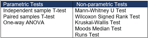
McNemar Test –

This test is basically a type of matched pair test and is used to analyze data before and after an event has occurred. It tells us whether there is a significant change in the data before and after the occurrence of any said event. Use McNemar’s Test with paired samples where the dependent variable is dichotomous.

Runs Test – This test is to determine whether the sequence of a series of events is random or not. Use one or two sample types depending on the data available at hand and the resources available. The two-sample test determines whether the two samples come from the same distribution of data or not.

Resampling Procedures – Works on the assumption that the original population distribution is the same as in the given sample. This helps us create a large number of samples from this pseudo-population and then in end draw valuable conclusions.

Additional Non-Parametric Hypothesis Tests

Apart from the above non-parametric test, some of the other examples of non-parametric tests used in our everyday lives are the Chi-square Test of Independence , Kolmogorov-Smirnov (KS) test, Kruskal-Wallis Test , Mood’s Median Test , Spearman’s Rank Correlation, Kendall’s Tau Correlation, Friedman Test and the Cochran’s Q Test.

Also, see one and two sample proportion non-parametric hypothesis tests , 1 Sample Sign Non Parametric Hypothesis Test ,

Advantages of Non-parametric tests

• Non-parametric tests are distribution free
• An added advantage is the reduction in the effect of outliers and variance heterogeneity on our results.
• It can be applied to nominal (such as sex, race, employment status, etc.) or ordinal scaled data ( on a 1-10 scale, 10 being delighted and 1 being extremely dissatisfied)
• Computations are easier than the parametric test
• Easy to understand and less time-consuming especially when the sample size is small

Disadvantages of Non-parametric tests

• The results that they provide may be less efficient or powerful compared to the results provided by the parametric tests.
• Non-parametric tests are useful and important in many cases, but it is difficult to compute manually.
• Results are usually more difficult to interpret than parametric tests
• Use Non-parametric tests for correlation studies
• Tests for equality of population medians – Mood’s Median, Mann Whitney, and Kruskal Wallis
• Non-Parametric Test of equality of population variances – Levene’s Test
• Levene’s test – makes an evaluation using a t-test http://en.wikipedia.org/wiki/Levene’s_test  (Levene’s test of equal variances)

Non-Parametric test videos

Six Sigma Black Belt Certification Non-Parametric Tests and Data Analysis Questions:

Question: A black belt would use non-parametric statistical methods when:

(A) knowledge of the underlying distribution of the population is limited (B) the measurement scale is either nominal or ordinal (C) the statistical estimation is required to have higher assurance (D) management requires substantial statistical analysis prior to implementing

Unlock Additional Members-only Content!

Thank you for being a member.

A: knowledge of the underlying distribution of the population is limited.

You use non-parametrics when you can’t identify or assume what kind of distribution you have so A is the easy choice. Also, you can eliminate b, c, and d as they have no bearing on the problem.

Comments (4)

I would believe the correct answer is B not A.

I can run a normality test to know if the data follow normal distribution or not, and that’s enough information to whether use non-parametric statistical methods.

However if the measurement scale is either ordinal or nominal, then by definition I have to use non-parametric statistical methods.

Thanks, Ahmed

Thanks for the question. This question comes from ASQ’s published practice exam and that is their provided answer.

I think it comes down to which is the best possible answer. While you are right in terms of B, A is the better answer as it is more encompassing.

Thanks for reaching out. I moved this conversation to the private member’s forum. I’ll follow up there.

As a reminder, please only discuss the questions from the practice exams in the member’s forum.

Leave a Reply Cancel reply

Your email address will not be published. Required fields are marked *

This site uses Akismet to reduce spam. Learn how your comment data is processed .

Insert/edit link

Enter the destination URL

Or link to existing content

Non-Parametric Test

Non-parametric test is a statistical analysis method that does not assume the population data belongs to some prescribed distribution which is determined by some parameters. Due to this, a non-parametric test is also known as a distribution-free test. These tests are usually based on distributions that have unspecified parameters.

A non-parametric test acts as an alternative to a parametric test for mathematical models where the nature of parameters is flexible. Usually, when the assumptions of parametric tests are violated then non-parametric tests are used. In this article, we will learn more about a non-parametric test, the types, examples, advantages, and disadvantages.

What is Non-Parametric Test in Statistics?

A non-parametric test in statistics does not assume that the data has been taken from a normal distribution . A normal distribution belongs to a parametrized family of probability distributions and includes parameters such as mean, variance, standard deviation, etc. Thus, a non-parametric test does not make assumptions about the probability distribution's parameters.

Non-Parametric Test Definition

A non-parametric test can be defined as a test that is used in statistical analysis when the data under consideration does not belong to a parametrized family of distributions. When the data does not meet the requirements to perform a parametric test, a non-parametric test is used to analyze it.

Reasons to Use Non-Parametric Tests

It is important to access when to apply parametric and non-parametric tests in order to arrive at the correct statistical inference. The reasons to use a non-parametric test are given below:

• When the distribution is skewed, a non-parametric test is used. For skewed distributions, the mean is not the best measure of central tendency, hence, parametric tests cannot be used.
• If the size of the data is too small then validating the distribution of the data becomes difficult. Thus, in such cases, a non-parametric test is used to analyze the data.
• If the data is nominal or ordinal, a non-parametric test is used. This is because a parametric test can only be used for continuous data.

Types of Non-Parametric Tests

Parametric tests are those that assume that the data follows a normal distribution. Examples include ANOVA and t-tests. There are many different methods available to perform a non-parametric test. These tests can also be used in hypothesis testing. Some common non-parametric tests are given as follows:

Mann-Whitney U Test

This non-parametric test is analogous to t-tests for independent samples. To conduct such a test the distribution must contain ordinal data. It is also known as the Wilcoxon rank sum test.

Null Hypothesis: \(H_{0}\): The two populations under consideration must be equal.

Test Statistic: U should be smaller of

\(U_{1} = n_{1}n_{2}+\frac{n_{1}(n_{1}+1)}{2}-R_{1}\) or \(U_{2} = n_{1}n_{2}+\frac{n_{2}(n_{2}+1)}{2}-R_{2}\)

where, \(R_{1}\) is the sum of ranks in group 1 and \(R_{2}\) is the sum of ranks in group 2.

Decision Criteria: Reject the null hypothesis if U < critical value.

Wilcoxon Signed Rank Test

This is the non-parametric test whose counterpart is the parametric paired t-test . It is used to compare two samples that contain ordinal data and are dependent. The Wilcoxon signed rank test assumes that the data comes from a symmetric distribution.

Null Hypothesis: \(H_{0}\): The difference in the median is 0.

Test Statistic: W. W is defined as the smaller of the sums of the negative and positive ranks.

Decision Criteria: Reject the null hypothesis if W < critical value.

This non-parametric test is the parametric counterpart to the paired samples t-test. The sign test is similar to the Wilcoxon sign test.

Test Statistic: The smaller value among the number of positive and negative signs.

Decision Criteria: Reject the null hypothesis if the test statistic < critical value.

Kruskal Wallis Test

The parametric one-way ANOVA test is analogous to the non-parametric Kruskal Wallis test. It is used for comparing more than two groups of data that are independent and ordinal.

Null Hypothesis: \(H_{0}\): m population medians are equal

Test Statistic: H = \(\left ( \frac{12}{N(N+1)}\sum_{1}^{m} \frac{R_{j}^{2}}{n_{j}}\right ) - 3(N+1)\)

where, N = total sample size, \(n_{j}\) and \(R_{j}\) are the sample size and the sum of ranks of the j th group

Decision Criteria: Reject the null hypothesis if H > critical value

Non-Parametric Test Example

The best way to understand how to set up and solve a hypothesis involving a non-parametric test is by taking an example.

Suppose patients are suffering from cancer. They are divided into three groups and different drugs were administered. The platelet count for the patients is given in the table below. It needs to be checked if the population medians are equal. The significance level is 0.05.

As the size of the 3 groups is not same the Kruskal Wallis test is used.

\(H_{0}\): Population medians are same

\(H_{1}\): Population medians are different

\(n_{1}\) = 5, \(n_{2}\) = 3, \(n_{3}\) = 4

N = 5 + 3 + 4 = 12

Now ordering the groups and assigning ranks

\(R_{1}\) = 18.5, \(R_{2}\) = 21, \(R_{3}\) = 38.5,

Substituting these values in the test statistic formula, \(\left ( \frac{12}{N(N+1)}\sum_{1}^{m} \frac{R_{j}^{2}}{n_{j}}\right ) - 3(N+1)\)

H = 6.0778.

Using the critical value table, the critical value will be 5.656.

As H < critical value, the null hypothesis is rejected and it is concluded that there is no significant evidence to show that the population medians are equal.

Difference between Parametric and Non-Parametric Test

Depending upon the type of distribution that the data has been obtained from both, a parametric test and a non-parametric test can be used in hypothesis testing. The table given below outlines the main difference between parametric and non-parametric tests.

Advantages and Disadvantages of Non-Parametric Test

Non-parametric tests are used when the conditions for a parametric test are not satisfied. In some cases when the data does not match the required assumptions but has a large sample size then a parametric test can still be used. Some of the advantages and disadvantages of a non-parametric test are listed as follows:

Advantages of Non-Parametric Test

The advantages of a non-parametric test are listed as follows:

• Knowledge of the population distribution is not required.
• The calculations involved in such a test are shorter.
• A non-parametric test is easy to understand.
• These tests are applicable to all data types.

Disadvantages of Non-Parametric Test

The disadvantages of a non-parametric test are given below:

• They are not as efficient as their parametric counterparts.
• As these are distribution-free tests the level of accuracy is reduced.

Related Articles:

• Summary Statistics
• Probability and Statistics
• T-Distribution

Important Notes on Non-Parametric Test

• A non-parametric test is a statistical test that is performed on data belonging to a distribution whose parameters are unknown.
• It is used on skewed distributions and the measure of central tendency used is the median.
• Kruskal Wallis test, sign test, Wilcoxon signed test and the Mann Whitney u test are some important non-parametric tests used in hypothesis testing.

Examples on Non-Parametric Test

Example 1: A surprise quiz was taken and the scores of 6 students are given as follows:

After giving a month's time to practice, the same quiz was taken again and the following scores were obtained.

Assigning signed ranks to the differences

\(H_{0}\): Median difference is 0. \(H_{1}\): Median difference is positive. W1: Sum of positive ranks = 17.5 W2: Sum of negative ranks = 3.5 As W2 < W1, thus, W2 is the test statistic. Now from the table, the critical value is 2. Since W2 > 2, thus, the null hypothesis cannot be rejected and it can be concluded that there is no difference between the scores of the two tests. Answer: Fail to reject the null hypothesis

\(H_{0}\): Two groups report same number of cases \(H_{1}\): Two groups report different number of cases \(R_{1}\) = 15.5, \(R_{2}\) = 39.5 \(n_{1}\) = \(n_{2}\) = 5 Using the formulas, \(U_{1} = n_{1}n_{2}+\frac{n_{1}(n_{1}+1)}{2}-R_{1}\) and \(U_{2} = n_{1}n_{2}+\frac{n_{2}(n_{2}+1)}{2}-R_{2}\) \(U_{1}\) = 24.5, \(U_{2}\) = 0.5 As \(U_{2}\) < \(U_{1}\), thus, \(U_{2}\) is the test statistic. From the table the critical value is 2 As \(U_{2}\) < 2, the null hypothesis is rejected and it is concluded that there is no evidence to prove that the two groups have the same number of sleepwalking cases. Answer: Null hypothesis is rejected

go to slide go to slide go to slide

Book a Free Trial Class

FAQs on Non-Parametric Test

What is a non-parametric test.

A non-parametric test in statistics is a test that is performed on data belonging to a distribution that has flexible parameters. Thus, they are also known as distribution-free tests.

When Should a Non-Parametric Test be Used?

A non-parametric test should be used under the following conditions.

• The distribution is skewed.
• The size of the distribution is small.
• The data is nominal or ordinal.

What is the Test Statistic Used for the Mann-Whitney U Non-Parametric Test?

The Mann Whitney U non-parametric test is the non parametric version of the sample t-test. The test statistic used for hypothesis testing is U . U should be smaller of \(U_{1} = n_{1}n_{2}+\frac{n_{1}(n_{1}+1)}{2}-R_{1}\) or \(U_{2} = n_{1}n_{2}+\frac{n_{2}(n_{2}+1)}{2}-R_{2}\)

What is the Test Statistic Used for the Kruskal Wallis Non-Parametric Test?

The parametric counterpart of the Kruskal Wallis non parametric test is the one way ANOVA test. The test statistic used is H = \(\left ( \frac{12}{N(N+1)}\sum_{1}^{m} \frac{R_{j}^{2}}{n_{j}}\right ) - 3(N+1)\).

What is the Test Statistic Used for the Sign Non-Parametric Test?

The smaller value among the number of positive and negative signs is the test statistic that is used for the sign non-parametric test.

What is the Difference Between a Parametric and Non-Parametric Test?

A parametric test is conducted on data that is obtained from a parameterized distribution such as a normal distribution. On the other hand, a non-parametric test is conducted on a skewed distribution or when the parameters of the population distribution are not known.

What are the Advantages of a Non-Parametric Test?

A non-parametric test does not rely on the assumed parameters of a distribution and is applicable to all data types. Furthermore, they are easy to understand.

• Number Theory
• Data Structures
• Cornerstones

Non-Parametric Tests

Wilcoxon rank sum test.

The Wilcoxon Rank Sum test is a non-parametric hypothesis test where the null hypothesis is that there is no difference in the populations (i.e., they have equal medians).

This test does assume that the two samples are independent, and both $n_1$ and $n_2$ are at least $10$. It should not be used if either of these assumptions are not met.

The test involves first ranking the data in both samples, taken together. Each data element is given a rank, $1$ through $n_1 + n_2$, from lowest to highest -- with ties resolved by ranking tied elements arbitrarily at first, and then replacing rankings of tied elements with the average rank of those tied elements.

So for example, ranking the data below $$\begin{array}{l|cccccccc} \textrm{Sample A} & 12 & 15 & 17 & 18 & 18 & 20 & 23 & 24\\\hline \textrm{Sample B} & 14 & 15 & 18 & 20 & 20 & 20 & 24 & 25\\ \end{array}$$ results in the following ranks $$\begin{array}{ccc} \textrm{value} & \textrm{initial rank} & \textrm{final rank}\\\hline 12 & 1 & 1\\ 14 & 2 & 2\\ 15 & 3 & 3.5\\ 15 & 4 & 3.5\\ 17 & 5 & 5\\ 18 & 6 & 7\\ 18 & 7 & 7\\ 18 & 8 & 7\\ 20 & 9 & 10.5\\ 20 & 10 & 10.5\\ 20 & 11 & 10.5\\ 20 & 12 & 10.5\\ 23 & 13 & 13\\ 24 & 14 & 14.5\\ 24 & 15 & 14.5\\ 25 & 16 & 16\\ \end{array}$$

Kruskal-Wallis Test (i.e., H Test)

The Kruskal-Wallis Test (named after William Kruskal and W. Allen Wallis) can be used to test the claim (a null hypothesis) that there is no difference in the populations (i.e., they have equal medians) when there are 3 or more independent samples, provided they meet the additional assumption that the sample sizes are all at least 5.

To perform the test, we first rank all of the samples together, and then add the ranks associated with each sample.

Letting $R_i$ be the sum of the ranks for sample $i$, of size $n_i$, $N$ be the sum of all sample sizes $n_i$, and $k$ be the number of samples, the following test statistic

This is a right-tailed test.

To see why this test statistic takes the form it does, consider the following:

Recall that a $\chi^2$-distribution is the distribution of a sum of the squares of independent standard normal random variables.

Under a presumption that the sample sizes, $n_i$, are not too small (remember, we required $n_i \ge 5$ for each sample), the $\overline{R_i}$ jointly will be approximately normally distributed.

( Note, we have relaxed our typical requirement that $n \ge 30$ down to $n \ge 5$ as the associated population is uniform. )

To make $H$ a sum of squares of standard normal random variables, we use $z$-scores for each observed average rank in a natural way:

Given the null hypothesis that there is no difference between the populations with regard to their medians, we can expect the ranks 1 to $N$ seen in the samples are distributed uniformly. Recalling that the expected value and variance of such a uniform distribution $X$ are given by $$E(X) = \frac{N+1}{2} \quad \quad \textrm{ and } \quad \quad Var(X) = (SD(X))^2 = \frac{N^2-1}{12}$$ we make the following substitutions:

Adding a factor of $(N-1)/N$ to correct bias (much like Bessel's correction), we have:

From here, we just use algebra to rewrite $H$ in a form more convenient for calculation:

• Math Article
• Non Parametric Test

Non-Parametric Test

Non-parametric tests are experiments that do not require the underlying population for assumptions. It does not rely on any data referring to any particular parametric group of probability distributions . Non-parametric methods are also called distribution-free tests since they do not have any underlying population.  In this article, we will discuss what a non-parametric test is, different methods, merits, demerits and examples of non-parametric testing methods.

Table of Contents:

• Non-parametric T Test
• Non-parametric Paired T-Test

Mann Whitney U Test

Wilcoxon signed-rank test, kruskal wallis test.

• Advantages and Disadvantages
• Applications

What is a Non-parametric Test?

Non-parametric tests are the mathematical methods used in statistical hypothesis testing, which do not make assumptions about the frequency distribution of variables that are to be evaluated. The non-parametric experiment is used when there are skewed data, and it comprises techniques that do not depend on data pertaining to any particular distribution.

The word non-parametric does not mean that these models do not have any parameters. The fact is, the characteristics and number of parameters are pretty flexible and not predefined. Therefore, these models are called distribution-free models.

Non-Parametric T-Test

Whenever a few assumptions in the given population are uncertain, we use non-parametric tests, which are also considered parametric counterparts. When data are not distributed normally or when they are on an ordinal level of measurement, we have to use non-parametric tests for analysis. The basic rule is to use a parametric t-test for normally distributed data and a non-parametric test for skewed data.

Non-Parametric Paired T-Test

The paired sample t-test is used to match two means scores, and these scores come from the same group. Pair samples t-test is used when variables are independent and have two levels, and those levels are repeated measures.

Non-parametric Test Methods

The four different techniques of parametric tests, such as Mann Whitney U test, the sign test, the Wilcoxon signed-rank test, and the Kruskal Wallis test are discussed here in detail. We know that the non-parametric tests are completely based on the ranks, which are assigned to the ordered data. The four different types of non-parametric test are summarized below with their uses, null hypothesis , test statistic, and the decision rule. 

Kruskal Wallis test is used to compare the continuous outcome in greater than two independent samples.

Null hypothesis, H 0 :  K Population medians are equal.

Test statistic:

If N is the total sample size, k is the number of comparison groups, R j is the sum of the ranks in the jth group and n j is the sample size in the jth group, then the test statistic, H is given by:

\(\begin{array}{l}H = \left ( \frac{12}{N(N+1)}\sum_{j=1}^{k} \frac{R_{j}^{2}}{n_{j}}\right )-3(N+1)\end{array} \)

Decision Rule: Reject the null hypothesis H 0 if H ≥ critical value

The sign test is used to compare the continuous outcome in the paired samples or the two matches samples.

Null hypothesis, H 0 : Median difference should be zero 

Test statistic: The test statistic of the sign test is the smaller of the number of positive or negative signs.

Decision Rule: Reject the null hypothesis if the smaller of number of the positive or the negative signs are less than or equal to the critical value from the table.

Mann Whitney U test is used to compare the continuous outcomes in the two independent samples. 

Null hypothesis, H 0 : The two populations should be equal.

If R 1 and R 2 are the sum of the ranks in group 1 and group 2 respectively, then the test statistic “U” is the smaller of:

\(\begin{array}{l}U_{1}= n_{1}n_{2}+\frac{n_{1}(n_{1}+1)}{2}-R_{1}\end{array} \)

\(\begin{array}{l}U_{2}= n_{1}n_{2}+\frac{n_{2}(n_{2}+1)}{2}-R_{2}\end{array} \)

Decision Rule: Reject the null hypothesis if the test statistic, U is less than or equal to critical value from the table.

Wilcoxon signed-rank test is used to compare the continuous outcome in the two matched samples or the paired samples.

Null hypothesis, H 0 : Median difference should be zero.

Test statistic: The test statistic W, is defined as the smaller of W+ or W- .

Where W+ and W- are the sums of the positive and the negative ranks of the different scores.

Decision Rule: Reject the null hypothesis if the test statistic, W is less than or equal to the critical value from the table.

Advantages and Disadvantages of Non-Parametric Test

The advantages of the non-parametric test are:

• Easily understandable
• Short calculations
• Assumption of distribution is not required
• Applicable to all types of data

The disadvantages of the non-parametric test are:

• Less efficient as compared to parametric test
• The results may or may not provide an accurate answer because they are distribution free

Applications of Non-Parametric Test

The conditions when non-parametric tests are used are listed below:

• When parametric tests are not satisfied.
• When testing the hypothesis, it does not have any distribution.
• For quick data analysis.
• When unscaled data is available.

Frequently Asked Questions on Non-Parametric Test

What is meant by a non-parametric test.

The non-parametric test is one of the methods of statistical analysis, which does not require any distribution to meet the required assumptions, that has to be analyzed. Hence, the non-parametric test is called a distribution-free test.

What is the advantage of a non-parametric test?

The advantage of nonparametric tests over the parametric test is that they do not consider any assumptions about the data.

Is Chi-square a non-parametric test?

Yes, the Chi-square test is a non-parametric test in statistics, and it is called a distribution-free test.

Mention the different types of non-parametric tests.

The different types of non-parametric test are: Kruskal Wallis Test Sign Test Mann Whitney U test Wilcoxon signed-rank test

When to use the parametric and non-parametric test?

If the mean of the data more accurately represents the centre of the distribution, and the sample size is large enough, we can use the parametric test. Whereas, if the median of the data more accurately represents the centre of the distribution, and the sample size is large, we can use non-parametric distribution.

• Share Share

Register with BYJU'S & Download Free PDFs

Register with byju's & watch live videos.

Hypothesis testing | Parametric and nonparametric tests

This article was published as part of the Data Science Blogathon

Introduction

Hypothesis testing is one of the most important concepts in Statistics that is widely used by Statistics , Machine learning engineers , Y Data scientists .

In hypothesis testing, statistical tests are used to check whether the null hypothesis is rejected or not rejected. Are Statistical tests assume null hypothesis no relationship or no difference between groups.

Then, in this article, we will discuss the statistical test for hypothesis testing, including parametric and nonparametric tests.

Table of Contents

1. What are parametric tests?

2. What are nonparametric tests?

3. Parametric tests for hypothesis tests

4. Nonparametric tests for hypothesis tests

• Chi squared

Mann-Whitney U test

Kruskal-wallis h test.

Let us begin,

Parametric tests

The basic principle behind parametric testing is that we have a fixed set of parameters that are used to determine a probabilistic model that can also be used in Machine Learning..

Parametric tests are those tests for which we have prior knowledge of the population distribution (namely, normal), or if not, we can easily approximate it to a normal distribution, which is possible with the help of the Central Limit Theorem.

The parameters to use the normal distribution are:

Finally, the classification of a test as parametric depends entirely on the assumptions of the population. There are many parametric tests available, some of which are the following:

• To find the confidence interval for the population means with the help of the known standard deviation.
• Determine the confidence interval for the population means together with the unknown standard deviation.
• Finding the confidence interval for the population variance.
• Finding the Confidence Interval for the Difference of Two Means, with an unknown standard deviation value.

Nonparametric tests

In nonparametric tests, we do not make any assumptions about the parameters for the given population or the population we are studying. In fact, these tests are not population dependent. Therefore, no fixed set of parameters available, and there is no distribution (normal distribution, etc.) of any kind available for use.

This is also why nonparametric tests are also called tests without distribution . Nowadays, nonparametric tests are gaining popularity and an influencing impact, some of the reasons behind this fame is:

• The main reason is that there is no need to be polite when using parametric tests.
• The second reason is that we don't need to make assumptions about the given population (the take) on which we are doing the analysis.
• Most of the non-parametric tests available are very easy to apply and understand as well, namely, complexity is very low.

Image source: Google images

1. It is a parametric test of hypothesis test based on Student's t distribution .

2. Essentially, it is about testing the significance of the difference of the mean values ​​when the sample size is small (namely, less than 30) and when the population standard deviation is not available.

3. Assumptions of this test:

• The population distribution is normal and
• Samples are random and independent.
• Sample size is small.
• The population standard deviation is unknown.

4. The 'U test’ Mann-Whitney is a nonparametric counterpart of the T test.

A T test can be:

One-sample T-test: Compare a sample mean with the population mean.

X is the sample mean

s is the standard deviation of the sample

North is the sample size

μ is the mean of the population

Two-sample T-test: Compare the means of two different samples.

X 1 is the sample mean of the first group

X 2 is the sample mean of the second group

S 1 is the standard deviation of the sample 1

S 2 is the standard deviation of the sample 2

Conclution:

• If the value of the test statistic is greater than the value in the table -> Reject the null hypothesis .
• If the value of the test statistic is less than the value in the table -> Don't reject the null hypothesis .

1. It is a parametric test of hypothesis test.

2. Used to determine if the means are different when the population variance is known and the sample size is large (namely, greater than 30).

• The population distribution is normal
• The sample size is large.
• The standard deviation of the population is known.

A Z test can be:

One sample Z test: Compare a sample mean with the population mean.

Two-sample Z test: Compare the means of two different samples.

σ 1 is the standard deviation of the population 1

σ 2 is the standard deviation of the population 2

1. It is a parametric test of hypothesis test based on Snedecor F distribution .

2. It is a test for the null hypothesis that two normal populations have the same variance.

3. An F test is considered a comparison of the equality of the sample variances.

4. The F statistic is simply a relationship of two variances.

5. It is calculated as:

F = s 1 2 /s 2 2

6. By changing the variance in the relationship, the F test has become a very flexible test. It can then be used to:

• Test general significance for a regression model.
• Compare the settings of different models and
• Test for equality of means.

7. Assumptions of this test:

• Samples are drawn randomly and independently.

1. Also called as Variation analysis , is a parametric test of hypothesis test.

2. It is an extension of the T test and the Z test.

3. Used to test the significance of differences in mean values ​​between more than two sample groups.

4. Use the F test to statistically test the equality of means and the relative variance between them.

5. Assumptions of this test:

• Homogeneity of the sample variance.

6. One-way ANOVA and two-way ANOVA are types.

7. F statistic = variance between the sample means / within-sample variance

Chi-square test

1. It is a non-parametric test of hypothesis testing.

2. As a nonparametric test, chi-square can be used:

• goodness of fit test.
• as a test of independence of two variables.

3. Helps to evaluate the goodness of fit between a set of theoretically observed and expected.

4. Makes a comparison between expected frequencies and observed frequencies.

5. The bigger the difference, the greater the chi-square value.

6. If there is no difference between the expected and observed frequencies, then the chi-square value is equal to zero.

7. It is also known as the “Goodness-of-fit test” which determines whether a particular distribution fits the observed data or not.

8. It is calculated as:

9. Chi-square is also used to test the independence of two variables.

10. Conditions for the chi-square test:

• Collect and record random observations.
• In the sample, all entities must be independent.
• Neither group should contain very few items, let's say less than 10.
• The reasonably large total number of items. Normally, should be at least 50, no matter how small the number of groups.

11. Chi-square as parametric test is used as test for population variance based on sample variance.

12. If we take each of a collection of sample variances, We divide them by the known population variance and multiply these ratios by (n-1), where n means the number of elements in the sample, we obtain the chi-square values.

13. It is calculated as:

2. This test is used to investigate whether two independent samples were selected from a population that has the same distribution..

3. It is a true nonparametric counterpart of the T-test and provides the most accurate estimates of significance., especially when sample sizes are small and the population does not have a normal distribution.

4. It is based on the comparison of each observation in the first sample with each observation in the other sample.

5. The test statistic used here is “U”.

6. The maximum value of “U” is' ​​n 1 *North 2 'And the minimum value is zero.

7. It is also known as:

• Mann-Whitney Wilcoxon test.
• Mann-Whitney Wilcoxon range test.

8. Mathematically, U is given by:

U 1 = R 1 – n 1 (North 1 +1) / 2

where 1 is the sample size for the sample 1, y R 1 is the sum of ranks in the Sample 1.

U 2 = R 2 – n 2 (North 2 +1) / 2

When consulting the tables of significance, the smallest values ​​of U 1 and you 2 They are used. The sum of two values ​​is given by,

U 1 + U 2 = {R 1 – n 1 (North 1 +1) / 2} + {R 2 – n 2 (North 2 +1) / 2}

Knowing that R 1 + R 2 = N (N + 1) / 2 and N = n 1 + n 2 , and doing some algebra, we find that the sum is:

U 1 + U 2 = n 1 *North 2

2. This test is used to compare two or more independent samples of the same or different sample sizes.

3. Extends the Mann-Whitney U test, which is used to compare only two groups.

4. The one-way ANOVA is the parametric equivalent of this test. And that is why it is also known as ‘ One-way ANOVA in ranges .

5. Use ranges instead of actual data.

6. It does not assume that the population is normally distributed.

7. The test statistic used here is “H”.

This completes today's discussion!!

Final notes

Thank you for reading!

Hope you enjoyed the article and increased your knowledge about statistical tests for hypothesis testing in statistics.

Please feel free to contact me about Email

Anything not mentioned or do you want to share your thoughts? Feel free to comment below and I'll get back to you.

For the remaining items, Ask the Link .

About the Author

Aashi goyal.

Nowadays, I am pursuing my Bachelor of Technology (B.Tech) in Electronic and Communication Engineering from Universidad Guru Jambheshwar (GJU), Hisar. I am very excited about the statistics, machine learning and deep learning.

The media shown in this article is not the property of DataPeaker and is used at the author's discretion.

Related Posts:

• Excel tips and tricks | Excel tips for data analysis
• The best resources for learning to program in MATLAB
• https://www.analyticsvidhya.com/blog/2020/02/cnn-vs-rnn-vs-mlp-analyzing-3-types-of-neural-networks-in-deep-learning/
• Threading in Python | What is Threading in Python?

Recent posts

Artificial Intelligence in Video: How New Technologies Are Changing Video Production?

IT profiles you should consider

How to record a screen on Windows computer?

¿Do you know the seniority levels?

Find Your Best Slip Rings and Rotary Joints Here

Posittion Agency: Advantages of link building for an online store

Subscribe to our newsletter.

We will not send you SPAM mail. We hate it as much as you.

The data always to the Peak

Hypothesis Testing and Non-parametric Test

• First Online: 25 January 2022

Cite this chapter

• Rajib Maity 3  

Part of the book series: Springer Transactions in Civil and Environmental Engineering ((STICEE))

594 Accesses

It is often required to make inferences about some parameters of the population based on the available data. Such inferences are very important in hydrology and hydroclimatology where the available data is generally limited. This is done through hypothesis testing. Hypothesis testing requires the knowledge of sampling distribution of different statistics and parameter estimation. Sampling distribution of mean and variance, and two types of parameter estimation — point estimation and interval estimation — are discussed at the starting of this chapter. Next, the hypothesis testing is taken up. Different cases are discussed elaborately with illustrative examples. Later, a few statistical tests are discussed that deal with the goodness of fit of a probability distribution to the data using the knowledge of hypothesis testing. Some of the commonly used non-parametric tests are also explained along with appropriate examples in the field of hydrology and hydroclimatology.

This is a preview of subscription content, log in via an institution to check access.

Access this chapter

• Available as PDF
• Read on any device
• Instant download
• Own it forever
• Available as EPUB and PDF
• Compact, lightweight edition
• Dispatched in 3 to 5 business days
• Free shipping worldwide - see info
• Durable hardcover edition

Tax calculation will be finalised at checkout

Purchases are for personal use only

Institutional subscriptions

Author information

Authors and affiliations.

Department of Civil Engineering, Indian Institute of Technology Kharagpur, Kharagpur, India

Rajib Maity

You can also search for this author in PubMed   Google Scholar

Corresponding author

Correspondence to Rajib Maity .

6.1 Electronic supplementary material

Below is the link to the electronic supplementary material.

Supplementary material 1 (zip 3 KB)

Rights and permissions.

Reprints and permissions

Copyright information

© 2022 The Author(s), under exclusive license to Springer Nature Singapore Pte Ltd.

About this chapter

Maity, R. (2022). Hypothesis Testing and Non-parametric Test. In: Statistical Methods in Hydrology and Hydroclimatology. Springer Transactions in Civil and Environmental Engineering. Springer, Singapore. https://doi.org/10.1007/978-981-16-5517-3_6

Download citation

DOI : https://doi.org/10.1007/978-981-16-5517-3_6

Published : 25 January 2022

Publisher Name : Springer, Singapore

Print ISBN : 978-981-16-5516-6

Online ISBN : 978-981-16-5517-3

eBook Packages : Engineering Engineering (R0)

Share this chapter

Anyone you share the following link with will be able to read this content:

Sorry, a shareable link is not currently available for this article.

Provided by the Springer Nature SharedIt content-sharing initiative

• Publish with us

Policies and ethics

• Find a journal
• Track your research

Non-Parametric Statistics in Python: Exploring Distributions and Hypothesis Testing

Non-parametric statistics do not assume any strong assumptions of the distribution, which contrasts with parametric statistics. Non-parametric statistics focus on ranks and signs along with minimal assumptions.

Non-parametric statistics focus on analyzing data without making strong assumptions about the underlying distribution. Python offers various methods for exploring data distributions, such as histograms, kernel density estimation (KDE), and Q-Q plots. Apart from this, non-parametric hypothesis testing techniques like the Wilcoxon rank-sum test, Kruskal-Wallis test, and chi-square test allow for inferential analysis without relying on parametric assumptions.

In this article, we have divided non-parametric statistics into two parts – Methods for Exploring the underlying distribution and Hypothesis Testing and Inference.

Recommended: How To Calculate Power Statistics?

Exploring Data Distributions

Exploration of distribution helps us visualize the data and pin it to a theoretical distribution. It also helps us summarize the stats.

This subheading will teach us about Histograms, Kernel Density Estimation, and Q-Q Plots. We will also implement each of them in Python.

Visualizing Data with Histograms

Histograms are used to visualize the distribution of numerical data. The histogram gives us the range and shows the frequency of the range. They are very similar to Bar charts. Let us understand it further with Python code.

Let us look at the output for the above code.

Estimating Probability Density with Kernel Density Estimation

Kernel Density Estimation (KDE) approximates the random variable’s probability density function (pdf). It provides us with continuous and much smoother visualization of the distribution. Let us look at the Python code for the same.

Let us look at the output of the above code.

Comparing Distributions with Q-Q Plots

Q-Q Plots or quantile=quantile plots are used to compare two probability distributions. They help us visualize whether two datasets came from some population or have the same distribution. Let us look at the Python code for the same.

Let us look at the output of the plot.

Now let us move on and see what are the methods for Hypothesis Testing and Inference.

Non-Parametric Hypothesis Testing and Inference

In Hypothesis testing and inference for non-parametric statistics, minimal assumptions about the underlying distribution are made and more focus is on rank-based statistics.

Under this subheading, we will learn about the Wilcoxon rank-sum, Krusal-Wallis, and Chi-square tests. Let us learn all of these with their Python implementation.

Comparing Means with Wilcoxon Rank-Sum Test

The Wilcoxon rank sum test, or the Mann-Whitney U test, is a non-parametric statistical test used to compare the means of two independent groups. In the code below, we have two datasets, and we want to conclude if there is any difference between the mean of the datasets. Let us look at the code below.

Let us look at its output.

Since the p-value is greater than 0.05, we can conclude that there is no difference between the mean of the datasets.

One-way ANOVA on ranks/Krusal Wallis Test

One-way ANOVA on ranks or Krusal-Wallis test is a non-parametric test to compare the mean of three or more independent groups. It does not assume normally distributed data. Let us look at the output code where we have assumed three datasets.

Let us look at the output of the code below.

We fail to reject the null hypothesis since the p-value is greater than 0.05.

Testing Categorical Variables with Chi-Square Test

The chi-square test tests the difference between observed and expected frequencies in one or more categorical variables. It is also used for goodness-of-fit tests or whether they are independent. Let us look at the code below.

Since the p-value is more than 0.05, we cannot conclude any dependence between datasets.

Here we go! Now you know what non-parametric tests are. In this article, we have learned about the exploration of distribution and hypothesis testing of data without considering any parameters. We also learned about different kinds of tests to compare different datasets.

Hope you enjoyed reading it!!

Recommended: Chi-square test in Python — All you need to know!!

Recommended: Python’s Influence on Cloud Computing Projects: Revealing the Statistics