l'aquila earthquake geography case study

Case Studies: The L'Aquila & Kashmir Earthquakes

Earthquakes in high income countries - l'aquila, italy.

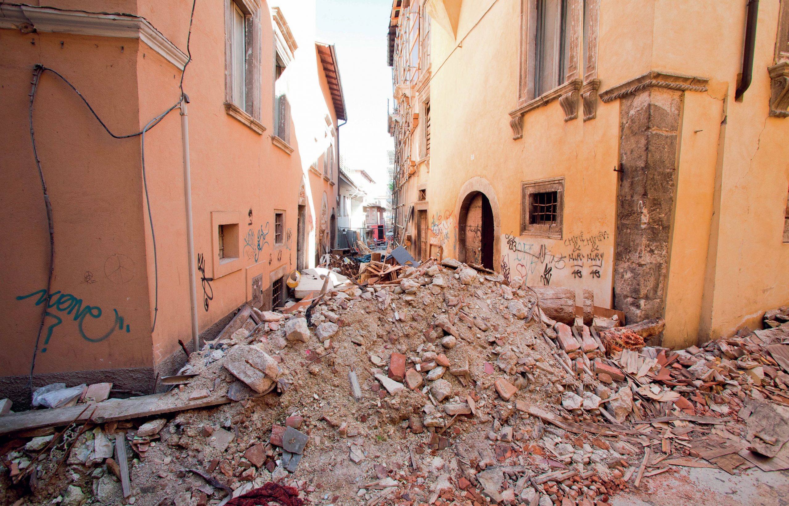
On the 6 th of April 2009, there was an earthquake with a magnitude of 6.3 in a town called L'Aquila in the Abruzzi region in Italy.

Primary effects - deaths and damage

• 308 people died and about 1,600 people were injured.
• More than 65,000 became homeless.
• The water supply into the Paganica (a town) was damaged, cutting them off from vital water supplies.

Secondary effects - aftershocks and infrastructure

• There were aftershocks that caused further damage after the initial earthquake.
• All telecommunications (phone) and electricity infrastructure was up and running in less than 24 hours.

Immediate responses - shelter and support

• Homeless people were given shelter, food, drinks, and medical attention. They also got free mobiles to communicate with their families.
• The army, medical personnel, and the fire department all helped clear the wreckage.
• The immediate response was helped by the fact that L'Aquila is closer than 100km to Rome and Italy is a relatively rich country.

Long-term responses - rebuilding

• The city centre was rebuilt to try to rehouse the 65,000 people who had become homeless.
• The inability of modern buildings to cope with earthquakes was investigated.
• 7 people were tried for manslaughter for not giving strong enough warnings about the earthquake.

Earthquake in Low Income Country - Kashmir, Pakistan

On the 8 th of October 2005, there was an earthquake with a magnitude of 7.6 in Pakistan (low-income country).

Primary effects of the Kashmir earthquake

• 79,000 people died and lots of buildings crumbled to the ground.
• It is hard to find an exact figure, but people estimate that 4 million people became homeless.
• Infrastructure was damaged. Millions of people had no clean water and no electricity.

Secondary effects of the Kashmir earthquake

• Landslides killed people and destroyed towns.
• Sewage pipes broke. This spread contaminated water and disease.
• The winter of 2005-2006 was very cold. 4 million people became homeless and lots of the homeless froze to death during the winter.

Immediate response to the Kashmir earthquake

• Charities and foreign governments sent funds, aid workers and helicopters.
• Charities gave out warm clothes, and tents, but a lot of support took a month to arrive because of the cold weather, damaged infrastructure, and the high number of people affected.

Long-term response to the Kashmir earthquake

• Thousands of people were relocated to new settlements, but 4 million people had been made homeless.
• The Pakistan government gave people money to try to rebuild their houses and homes, but because they were starving to death, they were forced to spend money on food instead.
• Thousands of people still lived in tents in 2015, a decade later.
• The government changed building regulations to try to stop this damage happening again.

Cause of the Kashmir earthquake

• Running through the middle of Pakistan is a collision plate boundary between the Eurasian and Indian plates, which means that Pakistan is prone to seismic activity.
• These plates have folded and forced each other upwards to form the Himalayan fold mountain range.
• The strain at this boundary was suddenly released on 8th October, 2005.

1 The Challenge of Natural Hazards

1.1 Natural Hazards

1.1.1 Types of Natural Hazards

1.1.2 Hazard Risk

1.1.3 Consequences of Natural Hazards

1.1.4 End of Topic Test - Natural Hazards

1.1.5 Exam-Style Questions - Natural Hazards

1.2 Tectonic Hazards

1.2.1 Tectonic Plates

1.2.2 Tectonic Plates & Convection Currents

1.2.3 Plate Margins

1.2.4 Volcanoes

1.2.5 Effects of Volcanoes

1.2.6 Responses to Volcanic Eruptions

1.2.7 Earthquakes

1.2.8 Earthquakes 2

1.2.9 Responses to Earthquakes

1.2.10 Case Studies: The L'Aquila & Kashmir Earthquakes

1.2.11 Earthquake Case Study: Chile 2010

1.2.12 Earthquake Case Study: Nepal 2015

1.2.13 Living with Tectonic Hazards 1

1.2.14 Living with Tectonic Hazards 2

1.2.15 End of Topic Test - Tectonic Hazards

1.2.16 Exam-Style Questions - Tectonic Hazards

1.2.17 Tectonic Hazards - Statistical Skills

1.3 Weather Hazards

1.3.1 Global Atmospheric Circulation

1.3.2 Surface Winds

1.3.3 UK Weather Hazards

1.3.4 Tropical Storms

1.3.5 Features of Tropical Storms

1.3.6 Impact of Tropical Storms 1

1.3.7 Impact of Tropical Storms 2

1.3.8 Tropical Storms Case Study: Katrina

1.3.9 Tropical Storms Case Study: Haiyan

1.3.10 UK Weather Hazards Case Study: Somerset 2014

1.3.11 End of Topic Test - Weather Hazards

1.3.12 Exam-Style Questions - Weather Hazards

1.3.13 Weather Hazards - Statistical Skills

1.4 Climate Change

1.4.1 Evidence for Climate Change

1.4.2 Causes of Climate Change

1.4.3 Effects of Climate Change

1.4.4 Managing Climate Change

1.4.5 End of Topic Test - Climate Change

1.4.6 Exam-Style Questions - Climate Change

1.4.7 Climate Change - Statistical Skills

2 The Living World

2.1 Ecosystems

2.1.1 Ecosystems

2.1.2 Ecosystem Cascades & Global Ecosystems

2.1.3 Ecosystem Case Study: Freshwater Ponds

2.2 Tropical Rainforests

2.2.1 Tropical Rainforests - Intro & Interdependence

2.2.2 Adaptations

2.2.3 Biodiversity of Tropical Rainforests

2.2.4 Deforestation

2.2.5 Case Study: Deforestation in the Amazon Rainforest

2.2.6 Sustainable Management of Rainforests

2.2.7 Case Study: Malaysian Rainforest

2.2.8 End of Topic Test - Tropical Rainforests

2.2.9 Exam-Style Questions - Tropical Rainforests

2.2.10 Deforestation - Statistical Skills

2.3 Hot Deserts

2.3.1 Overview of Hot Deserts

2.3.2 Biodiversity & Adaptation to Hot Deserts

2.3.3 Case Study: Sahara Desert

2.3.4 Desertification

2.3.5 Case Study: Thar Desert

2.3.6 End of Topic Test - Hot Deserts

2.3.7 Exam-Style Questions - Hot Deserts

2.4 Tundra & Polar Environments

2.4.1 Overview of Cold Environments

2.4.2 Adaptations in Cold Environments

2.4.3 Biodiversity in Cold Environments

2.4.4 Case Study: Alaska

2.4.5 Sustainable Management

2.4.6 Case Study: Svalbard

2.4.7 End of Topic Test - Tundra & Polar Environments

2.4.8 Exam-Style Questions - Cold Environments

3 Physical Landscapes in the UK

3.1 The UK Physical Landscape

3.1.1 The UK Physical Landscape

3.2 Coastal Landscapes in the UK

3.2.1 Types of Wave

3.2.2 Weathering & Mass Movement

3.2.3 Processes of Erosion & Wave-Cut Platforms

3.2.4 Headlands, Bays, Caves, Arches & Stacks

3.2.5 Transportation

3.2.6 Deposition

3.2.7 Spits, Bars & Sand Dunes

3.2.8 Case Study: Landforms on the Dorset Coast

3.2.9 Types of Coastal Management 1

3.2.10 Types of Coastal Management 2

3.2.11 Coastal Management Case Study - Holderness

3.2.12 Coastal Management Case Study: Swanage

3.2.13 Coastal Management Case Study - Lyme Regis

3.2.14 End of Topic Test - Coastal Landscapes in the UK

3.2.15 Exam-Style Questions - Coasts

3.3 River Landscapes in the UK

3.3.1 The River Valley

3.3.2 River Valley Case Study - River Tees

3.3.3 Erosion

3.3.4 Transportation & Deposition

3.3.5 Waterfalls, Gorges & Interlocking Spurs

3.3.6 Meanders & Oxbow Lakes

3.3.7 Floodplains & Levees

3.3.8 Estuaries

3.3.9 Case Study: The River Clyde

3.3.10 River Management

3.3.11 Hard & Soft Flood Defences

3.3.12 River Management Case Study - Boscastle

3.3.13 River Management Case Study - Banbury

3.3.14 End of Topic Test - River Landscapes in the UK

3.3.15 Exam-Style Questions - Rivers

3.4 Glacial Landscapes in the UK

3.4.1 Erosion

3.4.2 Landforms Caused by Erosion

3.4.3 Landforms Caused by Transportation & Deposition

3.4.4 Snowdonia

3.4.5 Land Use in Glaciated Areas

3.4.6 Tourism in Glacial Landscapes

3.4.7 Case Study - Lake District

3.4.8 End of Topic Test - Glacial Landscapes in the UK

3.4.9 Exam-Style Questions - Glacial Landscapes

4 Urban Issues & Challenges

4.1 Urban Issues & Challenges

4.1.1 Urbanisation

4.1.2 Urbanisation Case Study: Lagos

4.1.3 Urbanisation Case Study: Rio de Janeiro

4.1.4 UK Cities

4.1.5 Case Study: Urban Regen Projects - Manchester

4.1.6 Case Study: Urban Change in Liverpool

4.1.7 Case Study: Urban Change in Bristol

4.1.8 Sustainable Urban Life

4.1.9 End of Topic Test - Urban Issues & Challenges

4.1.10 Exam-Style Questions - Urban Issues & Challenges

4.1.11 Urban Issues -Statistical Skills

5 The Changing Economic World

5.1 The Changing Economic World

5.1.1 Measuring Development

5.1.2 Classifying Countries Based on Wealth

5.1.3 The Demographic Transition Model

5.1.4 Physical & Historical Causes of Uneven Development

5.1.5 Economic Causes of Uneven Development

5.1.6 How Can We Reduce the Global Development Gap?

5.1.7 Case Study: Tourism in Kenya

5.1.8 Case Study: Tourism in Jamaica

5.1.9 Case Study: Economic Development in India

5.1.10 Case Study: Aid & Development in India

5.1.11 Case Study: Economic Development in Nigeria

5.1.12 Case Study: Aid & Development in Nigeria

5.1.13 Economic Development in the UK

5.1.14 Economic Development UK: Industry & Rural

5.1.15 Economic Development UK: Transport & North-South

5.1.16 Economic Development UK: Regional & Global

5.1.17 End of Topic Test - The Changing Economic World

5.1.18 Exam-Style Questions - The Changing Economic World

5.1.19 Changing Economic World - Statistical Skills

6 The Challenge of Resource Management

6.1 Resource Management

6.1.1 Global Distribution of Resources

6.1.2 Food in the UK

6.1.3 Water in the UK 1

6.1.4 Water in the UK 2

6.1.5 Energy in the UK

6.1.6 Resource Management - Statistical Skills

6.2.1 Areas of Food Surplus & Food Deficit

6.2.2 Food Supply & Food Insecurity

6.2.3 Increasing Food Supply

6.2.4 Case Study: Thanet Earth

6.2.5 Creating a Sustainable Food Supply

6.2.6 Case Study: Agroforestry in Mali

6.2.7 End of Topic Test - Food

6.2.8 Exam-Style Questions - Food

6.2.9 Food - Statistical Skills

6.3.1 The Global Demand for Water

6.3.2 What Affects the Availability of Water?

6.3.3 Increasing Water Supplies

6.3.4 Case Study: Water Transfer in China

6.3.5 Sustainable Water Supply

6.3.6 Case Study: Kenya's Sand Dams

6.3.7 Case Study: Lesotho Highland Water Project

6.3.8 Case Study: Wakel River Basin Project

6.3.9 Exam-Style Questions - Water

6.3.10 Water - Statistical Skills

6.4.1 Global Demand for Energy

6.4.2 Factors Affecting Energy Supply

6.4.3 Increasing Energy Supply: Renewables

6.4.4 Increasing Energy Supply: Non-Renewables

6.4.5 Carbon Footprints & Energy Conservation

6.4.6 Case Study: Rice Husks in Bihar

6.4.7 Exam-Style Questions - Energy

6.4.8 Energy - Statistical Skills

Jump to other topics

Unlock your full potential with GoStudent tutoring

Affordable 1:1 tutoring from the comfort of your home

Tutors are matched to your specific learning needs

30+ school subjects covered

Responses to Earthquakes

Earthquake Case Study: Chile 2010

• Open access
• Published: 23 March 2020

Lessons from April 6, 2009 L’Aquila earthquake to enhance microzoning studies in near-field urban areas

• Giovanna Vessia 1 ,
• Mario Luigi Rainone 1 ,
• Angelo De Santis 2 &
• Giuliano D’Elia 1  

Geoenvironmental Disasters volume  7 , Article number:  11 ( 2020 ) Cite this article

2541 Accesses

2 Citations

2 Altmetric

Metrics details

This study focuses on two weak points of the present procedure to carry out microzoning study in near-field areas: (1) the Ground Motion Prediction Equations (GMPEs), commonly used in the reference seismic hazard (RSH) assessment; (2) the ambient noise measurements to define the natural frequency of the near surface soils and the bedrock depth. The limitations of these approaches will be discussed throughout the paper based on the worldwide and Italian experiences performed after the 2009 L’Aquila earthquake and then confirmed by the most recent 2012 Emilia Romagna earthquake and the 2016–17 Central Italy seismic sequence. The critical issues faced are (A) the high variability of peak ground acceleration (PGA) values within the first 20–30 km far from the source which are not robustly interpolated by the GMPEs, (B) at the level 1 microzoning activity, the soil seismic response under strong motion shaking is characterized by microtremors’ horizontal to vertical spectral ratios (HVSR) according to Nakamura’s method. This latter technique is commonly applied not being fully compliant with the rules fixed by European scientists in 2004, after a 3-year project named Site EffectS assessment using AMbient Excitations (SESAME). Hereinafter, some “best practices” from recent Italian and International experiences of seismic hazard estimation and microzonation studies are reported in order to put forward two proposals: (a) to formulate site-specific GMPEs in near-field areas in terms of PGA and (b) to record microtremor measurements following accurately the SESAME advice in order to get robust and repeatable HVSR values and to limit their use to those geological contests that are actually horizontally layered.

Introduction

On April 6, 2009, at 1:32 a.m. (local time) an M w 6.3 earthquake with shallow hypocentral depth (8.3 km) hit the city of L’Aquila and several municipalities within the Aterno Valley. This earthquake can be considered one of the most mournful seismic event in Italy since 1980 although its magnitude was moderately-high: 308 fatalities and 60.000 people displaced (data source http://www.protezionecivile.it ) and estimated damages for 1894 M€ (data source http://www.ngdc.noaa.gov ). These numbers showed how dangerous can be an unexpected seismic event in urbanized territories where no preventive actions have been addressed to reduce seismic risk. Hence, meanwhile, some actions were implementing in the post-earthquake time such as updating the reference Italian hazard map (by the Decree OPCM n. 3519 on 28 April 2006) and drawing microzoning maps to be used in the reconstruction stage, two major earthquakes struck the Emilia Romagna Region (in the Northern part of Italy), causing 27 deaths and widespread damage. The first, with M w 6.1, occurred on 20 May at 04:03 local time (02:03 UTC) and was located at about 36 km north of the city of Bologna. Then, a second major earthquake (M w 5.9) occurred on 29 May 2012, in the same area, causing widespread damage, particularly to buildings already weakened by the 20 May earthquake. Later on, the 2016–17 Central Italy Earthquake Sequence occurred, consisting of several moderately-high magnitude earthquakes between M w 5.5 and M w 6.5, from Aug 24, 2016, to Jan 18, 2017, each centered in a different but close location and with its own sequences of aftershocks, spanning several months. The seismic sequence killed about 300 people and injured the other 396. Worldwide, several other strong earthquakes (eg. 1998 Northridge earthquake, 2004 Parkfield earthquake, 2010 Canterbury and 2011 and 2017 Christchurch earthquakes, 2018 Sulawesi earthquake) produced devastating effects in the same time span. All these events show the need to carry out efficient microzoning studies to plan vulnerability reductions of urban structures and promoting the resilience of the human communities in seismic territories. After the 2009 L’Aquila earthquake, the microzoning studies have been introduced in Italy by law and the Guidelines for Seismic Microzonation (ICMS 2008 ) have been issued to accomplish these studies according to the most updated international scientific findings. These guidelines provide the local administrators with an efficient tool for seismic microzoning study to predicting the subsoil behavior under seismic shaking. Unfortunately, the ICMS does not give special recommendations for urbanized near field areas (NFAs). The microzoning activity concerning urbanized territories as suggest by ICMS ( 2008 ) is made up of four steps:

Estimating the reference seismic hazard to provide the input peak horizontal ground acceleration (PGA) at each point on the national territory and the normalized response spectrum at each site.

Dynamic characterization of soil deposits overlaying the seismic bedrock at each urban center in order to draw the microzoning maps (MM) at three main knowledge levels.

The Level 1 MM consists of geo-lithological maps of the surficial deposits that show typical successions and the amplified frequency map drawn through the measurements of microtremors elaborated by horizontal to vertical spectral ratio HVSR Nakamura’s technique. Nakamura’s method ( 1989 ), the horizontal to vertical noise components are calculated to derive the natural frequency of surficial soft deposits and their thickness.

The Level 2/3 MM consists of drawing maps after performing the numerical analyses of (a) seismic local amplification factors in terms of acceleration FA and velocity FV; (b) liquefaction potential LP and (c) permanent displacements due to seismically induced slope instability.

After 10 years of training the ICMS and the related methods, it is now the time to start analyzing some arisen weak points. Starting from the large data acquired worldwide on recent strong motion earthquakes, the experiences developed in seismic hazard assessment, and the site-specific seismic response characterization carried out by the writing authors after the 2009 L’Aquila earthquake, the aforementioned weak points (related to some aspects of the steps 1 and 3) are hereinafter discussed and some proposals are made to improve the efficiency of the microzoning studies especially in NFAs.

In this paper, after a brief background section on the procedures to accomplish the reference seismic hazard assessment (background section), the methods to calculate the Ground Motion Prediction Equations (GMPEs) and the HVSR (Nakamura’s method) are briefly recalled in section 2. Then in section 3, the results from observations of recorded peak ground acceleration (PGA) and pseudo-spectral acceleration (PSA) values within the NFAs from the L’Aquila earthquake and other worldwide strong earthquakes have been discussed. In addition, some applications of Nakamura’s procedure to characterize the natural frequency of the sites throughout the Aterno Valley have been discussed. Finally, in the conclusion section, some relevant points drawn from the discussed microzoning experiences have been highlighted to improve the efficiency of the microzonation studies in urban centers especially located in NFAs.

Background on seismic hazard assessment

Several theoretical and experimental studies performed worldwide in the last 50 years (see Kramer 1996 and the reference herein), highlighted that seismic shaking intensity is due to the magnitude of the earthquake generated at the source, to the travel paths of the seismic waves from the source to the buried or outcropping bedrock (that is called reference seismic hazard RSH) and the additional phenomena of local amplification or de-amplification take place where soil deposits overlay the rocky bedrock, named local seismic response LSR (Paolucci 2002 ; Vessia and Venisti 2011 ; Vessia et al. 2011 ; Vessia and Russo 2013 ; Vessia et al. 2013 , 2017 ; Boncio et al. 2018 , among others). The RSH maps drawn worldwide on national territories do not take into account the results of LSR studies.

The pioneering work by Signanini et al. ( 1983 ) after the 1979 Friuli earthquake confirmed the observations on the ground: local seismic effects could enlarge the referenced hazard at a site by 2–3 times in terms of MCS scale Intensity but also in PGA values owing to the local morphological and stratigraphic settings. Such RSL is particularly evident in near field areas, from then on named NFAs. The NFAs have been defined among others by Boore ( 2014a ) as the Fault Damage Zones. These areas cannot be uniquely identified depending on the source rupture mechanisms, the surficial soil deposits and the multiple calculation methods used for measuring the distance between the seismic stations and the source. Especially in these areas, about the first 30 km aside the source, spot-like amplifications are the common amplification pattern captured through the Maximum Intensity Felt maps. These maps estimate the differentiated damages suffered by buildings and urban structures by means of the Macroseismic Intensity scale (e.g. Mercalli-Cancani-Sieberg MCS scale, European Macroseismic scale EMS, Modified Mercalli Intensity MMI scale). One of the Maximum Intensity Felt maps on the Italian territory was drawn by Boschi et al. ( 1995 ). They took into account the seismic events that occurred from 1 to 1992 AD with a minimum intensity felt of VI MCS. This latter value is the one commonly used to highlight those areas where seismic events caused relevant damages to dwellings and infrastructures, ranging from severe damages to collapse. Boschi et al. ( 1995 ) map is reported in Fig.  1 : it showed IX-X MCS at L’Aquila district based on historical earthquakes that are in agreement with the seismic intensity map drawn by Galli and Camassi ( 2009 ) after the mainshock of 2009 L’Aquila earthquake. This map is also in very good agreement with other recent earthquakes such as the 2012 Emilia Romagna and 2016–17 Central Italy earthquakes (Fig. 1 ). Moreover, Boschi et al. ( 1995 ), Midorikawa ( 2002 ) and more recently, Paolini et al. ( 2012 ) proposed a direct use of the Maximum Felt Intensity maps to highlight those areas where the reference seismic hazard is largely increased by the local amplificated responses of soil deposits, that is the NFAs.

Italian Maximum Intensity felt map (After Boschi et al. 1995 , modified) with the areas of two recent Italian earthquake sequences considered in the present work

The most used method to perform the reference seismic hazard assessment has been conceived in the late ‘60s. It is Cornell’s method ( 1968 ) that was implemented into a numerical code by Mc Guire ( 1978 ). Cornell ( 1968 ) introduced the Probabilistic Seismic Hazard Assessment (PSHA) method to carry out the reference seismic hazard at a site considering the contribution of the seismic source and the travel path of the seismic waves by considering the uncertainties related to these estimations. This method consists of four steps (Kramer 1996 ), as illustrated in Fig.  2 :

STEP 1. To identify the seismogenic sources as single faults and faulting regions in terms of magnitude amplitude generated at different time spans. The probabilistic approach to such a characterization needs to know the rate of the earthquake at different magnitudes at the site and the spatial distribution of the fault segment or the source volume that can be activated.

STEP 2_1. To calculate the seismic rate in a region the Gutenberg-Richter law is used, where a and b coefficients are drawn by interpolating numerous data from a database of seismic events (instrumental and non-instrumental) available for a limited number of source areas and affected by the lack of completeness distortions. The earthquake occurrence probability is estimated by means of a Poisson distribution over time that is independent of the time span of the last strong seismic event.

STEP 2_2. To calculate the spatial distribution of the seismic events alongside a fault zone is a character difficult to get known and the spatial distribution of earthquake sources within a seismogenic area is commonly assumed uniformly distributed.

STEP 3. To define the ground motion prediction equations GMPEs that enable to predict, at different magnitude ranges, the decrease with the distance from the seismic source of the strong motion parameter assumed to be representative of the earthquake at a site.

STEP 4. To calculate the probability of exceedance of a target shaking value of the considered ground motion parameter, i.e. PGA, in a time span at a chosen site, due to the contribution of different seismogenic sources.

Cornell’s probabilistic seismic hazard assessment (PSHA) explained in four steps. The blue house represents the site under study

The previous 4 steps attempt to take into account several sources of uncertainties, such as the limited knowledge about the fault activity, the qualitative and documental estimations of the past earthquake effects at the sites, the lack of completeness of the seismic catalogs (meaning that the database of the seismic events is populated by several data related to both low and high magnitude ones) and the dependency among the recorded strong seismic events. In addition, the distortions in Gutenberg-Richter law, defined for different regions worldwide and the uncertainties related to the GMPEs can generate underestimations of the seismic shaking parameters (i.e. PGA) at specific sites where local seismic effects are relevant (Paolucci 2002 ; Vessia and Venisti 2011 ; Vessia and Russo 2013 ; Vessia et al. 2013 ; Yagoub 2015 ; Miyajima et al. 2019 ; Lanzo et al. 2019 ; among others). Logic trees are commonly used to take into account different formulations of GMPEs and several Gutenberg-Richter rates of magnitude occurrence (Kramer 1996 ).

Molina et al. ( 2001 ) pointed out that the PSHA has its strength in the systematic parameterization of seismicity and the way in which also epistemic uncertainties are carried out through the computations into the final results.

Recently, alternative approaches to PSHA calculation have been suggested, such as through extensions of the zonation method (Frankel 1995 ; Frankel et al. 1996 , 2000 ; Perkins 2000 ) where multiple source zones, parameter smoothing and quantification of geology and active faults have been successfully applied. The Frankel et al. ( 1996 ) method applied a Gaussian function to smooth a-values (within Gutenberg-Richter law) from each zone, thereby being a forerunner for the later zonation-free approaches of Woo ( 1996 ). This latter approach tries to amalgamate statistical consistency with the empirical knowledge of the earthquake catalogue (with its fractal character) into the computation of seismic hazard. Furthermore, Jackson and Kagan ( 1999 ) developed a non-parametric method with a continuous rate-density function (computed from earthquake catalogues) used in earthquake forecasting. Nonetheless, all these methods need a function to propagate the strong motion parameter values from the source to the site under study. To this end, the GMPEs are built by interpolating large databases of seismic records (related to specific geographical and tectonic environments worldwide), taking into account the contributions of the earthquake magnitude M and the distance to the seismic source R , according to the following form (Kramer 1996 ):

where Y is the ground motion parameter, commonly the peak ground horizontal acceleration PGA or the spectral acceleration SA at fixed period; S i is related to the source and site: they are the refinement terms due to the enlargement of the seismic databases and the possibility of drawing specific regional GMPEs.

The uncertainty of GMPEs in near field areas

Several examples of GMPEs are provided in literature (Kramer 1996 among others) while a recent throughout review of several possible formulations of GMPEs used in the USA can be found at the Pacific Earthquake Engineering Research center PEER website http://peer.berkeley.edu/publications/peer_reports_complete.html . In Italy, the GMPEs are built based on the PGAs drawn from the Italian shape wave database of strong motion events (Faccioli 2012 ; Bindi et al. 2011 , 2014 ; Cauzzi et al. 2014 ). Commonly, the PGA values represent the strong motion parameter used in microzoning studies but the related GMPEs are highly uncertain especially in the first tens of kilometers as shown in Fig.  3 a (Faccioli 2012 ) and Fig.  4 a (Boore 2013 ). According to Boore ( 2013 , 2014a ), fault zone records show significant variability in amplitude and polarization of PGA, SA especially at low periods (as shown in Fig. 4 a) and magnitude saturation beyond M w 6, although the causes of this variability are not easy to be unraveled. The main drawback of the GMPEs is the weakness of their predictivity at a short distance from the seismic source due to two main issues affecting the NFAs worldwide:

a few seismic stations installed;

highly scattered measures of strong motion parameters, especially in terms of accelerations (i.e. PGA, SA, etc) (Fig. 2 , step 3), that do not show any decreasing trend with distance.

a Ground Motion Prediction Equation (GMPE) of PGA versus the minimum source-to-site distance (After Faccioli 2012 , modified): a band of uncertainty (grey) of GMPEs proposed by Faccioli et al. ( 2010 ). b 2008 Boore and Atkinson ground motion prediction equation (BA08 GMPE) of PGA based on data collected in United States for Magnitude 7.3 M w , strike-slip fault type and V S30 equal to 255 m/s: solid line is the mean equation; dashed lines represent the confidence interval at one standard deviation (After Boore 2013 , modified)

a Measures of PSA during the Parkfield earthquake 2004 (6 M w ) are reported near the active fault at the measure seismic stations (After Boore 2014b , modified); b Onna sector of Aterno River Valley: the records are for an aftershock of 3.2 Ml

The PGA spatial uncertainties have been observed after several recent strong earthquakes, such as 2009 L’Aquila earthquake (Lanzo et al. 2010 ; Bergamaschi et al. 2011 ; Di Giulio et al. 2011 ), 2011 Christchurch and 2010 Darfield earthquakes in New Zealand (Bradley and Cubrinovski 2011 ) (Fig.  5 ), 2012 Emilia Romagna earthquake in Italy, 1994 Northridge earthquake in USA (Boore 2004 ) and 2013 Fivizzano earthquake (Fig. 5 ). In the case of the 2009 L’Aquila earthquake (Fig. 4 b), the areal distribution of PGAs around the source seems to be highly random although they show that the most dramatic increase occurs where thick soft sediments are met over rigid bedrocks or where bedrock basin shapes can be recognized. This latter traps the seismic waves and caused longer duration accelerograms with increased amplitudes at short and moderate periods (lower than 2 s) (Rainone et al. 2013 ).

Horizontal and vertical PGA values recorded within the first 20 km epicenter distance during 1) 22 February 2011 Christchurch earthquake (6.3 M w ) (square) and 2) 21 June 2013 Fivizzano earthquake (5.1 M w ) (triangle)

The GMPEs based on PGAs tend to saturate for large earthquakes as the distance from the fault rupture to the observation point decreases. Boore ( 2014b ) showed that the PGA parameter is a poor measure of the ground-motion intensity due to its non-unique correspondence to the frequency and acceleration content of the shaking waves (Fig. 4 ), especially at high frequencies. Furthermore, Bradley and Cubrinovski ( 2011 ) and Boore ( 2004 ) stated that the influence on the amplitude and shape response by local surface geology and geometrical conditions is noted to be much more relevant than the forward directivity and the source-site path on spectral accelerations in near field areas and for periods shorter than 3 s.

Thus, the GMPEs of PGAs within the NFAs are highly uncertain and cumbersome to be predicted even when fitted on single seismic events as shown in Fig. 5 (Bradley and Cubrinovski 2011 ; Faccioli 2012 ; Boore 2014b ). Faccioli ( 2012 ) evidenced 100% of the coefficient of variation about the mean trend of PGA GMPE versus source-to-site distance (Fig. 3 a). This GMPE was built based on the ITACA 2010 database (Luzi et al. 2008 , http://itaca.mi.ingv.it/ItacaNet_30/#/home ) that collects Italian strong motion shape waves. It is worth noticing that within the first tens of kilometers from the source, these data indicate that the GMPEs are not accurate in predicting the PGA values. To avoid the pitfalls in GMPEs based on peak parameters, integral ground motion parameters have been proposed in the literature (Kempton and Stewart 2006 ; Abrahamson and Silva 2008 ; Campbell and Bozorgnia 2012 ), such as Arias intensity (AI) and cumulative absolute velocity (CAV). In addition, Hollenback et al. ( 2015 ) and Stewart et al. ( 2015 ) formulated new generation GMPEs based on median ground-motion models as part of the Next Generation Attenuation for Central and Eastern North America project. They provided a set of adjustments to median GMPEs that are necessary to incorporate the source depth effects and the rupture distances in the range from 0 to 1500 Km. Moreover, the preceding authors suggest a distinct expression for the GMPE at short-distance to the source (by 10 km), that is:

where R RUP is the rupture distance, that is the closest distance to the earthquake rupture plane (km); c 1 and c 2 are the regression coefficients and h is a “fictitious depth” used for ground-motion saturation at close distances.

Ambient noise measures elaborated by means of the Nakamura horizontal to vertical ratio HVSR

In 1989 Nakamura proposed to use the ambient noise measurements to derive a seismic property of a site, that is the frequency range of amplification, through the spectral ratio of horizontal H and vertical V ambient vibration (microtremors) components of the recorded signals. If the site does not amplify, the ratio H/V is equal to 1. The Nakamura method shows the advantage to solve the troublesome issue to find out a reference site. In fact, it considers the vertical component as the one that is not modified by the site where horizontal subsoil layers are set and SH seismic waves represent the ambient noise signal content in a quite site (far from urban or industrial areas). This latter is the reference signal whereas the horizontal component is the only one that can be affected by the amplifying properties of the soils. As a matter of fact, Nakamura assumed that:

locally random distributed sources of microtremors generate not directional signals almost made up of shear horizontal or Rayleigh waves;

the microtremors are confined in the surficial layers because the subsoil is made up of soft layered sediments overlaying a rigid seismic bedrock.

A relevant implication of the Nakamura method is that the peaks of the ratio H/V are related to the presence of high acoustic impedance contrast at the depth h that can be derived by the following expression:

where V S is the mean value of the measured shear wave velocity profile and f o is the amplified frequency measured by means of the noise measurement.

The fundamental rules to perform a correct ambient noise recording was provided by the European research project named SESAME (Bard and the WG 2004 ) that analyzed the possible drawbacks of the simple model introduced by the Nakamura method and issued guidelines that offer important recommendations regarding the places where the method can be successfully used in urbanized areas. The given recommendations are based on a rather strict set of criteria, that are essentially composed of (1) experimental conditions and (2) criteria for gaining reliable results (Table 1 ).

As can be seen from Table 1 , the recommendations are focused on the weather conditions that influence the quality of the noise measurements and they highlight the need to record at distance from structures, trees, slopes because all these items affect the records. Unfortunately, it is not possible to quantify the minimum distance from the structure where the influence is negligible, as this distance depends on too many external factors (structure type, wind strength, soil type, etc.). Furthermore, related to the measurement spacing, SESAME guidelines suggest to never use a single measurement point to derive f 0 value, make at least three measurement points. This latter advice is often disregarded.

An interesting alternative way to apply the HVSR method is to investigate the “heavy tails” of its statistical distribution that is like that of a critical system (Signanini and De Santis 2012 ). This is likely indicative of the strong non-linear properties of rocks forming the uppermost crust resulting in a power-law trend.

However, the Nakamura technique has been introduced in microzoning studies at Level 1 in Italy (ICMS 2008 ) to draw the natural frequency map of urban sites but limitations to suitable sites have not been prescribed. Although the Nakamura method seems to be simple, lost cost and short time consuming, the suitable sites where it can be applied are few, especially in urban centers. This type of indirect investigation method is not applicable in complex geological contexts (e.g. buried inclined fold settings) and is not easily handled for the difficulties in reproducing the same measurements under variable site conditions and noise sources and acquisitions performed by different operators even at the same site.

Rainone et al. ( 2018 ) undertook a thorough study on the effectiveness of HVSR in predicting amplification frequencies at two Italian urban areas characterized by different subsoil setting and noise distribution. Results from this study show that HVSR works well only where horizontally layered sediments overlay a rigid bedrock: these conditions are the most relevant and the most influential on the predictivity of the actual f o measured values.

Results and discussion

A new proposal for gmpes in near field areas.

Recently, a study to formulate ad hoc GMPEs for PGAs within NFAs of the Central Italy Apennine sector has been performed. Only horizontal PGA values measured from seismic stations set on A and A* soil category (V s  ≥ 800 m/s), generated by seismic events with M w ranging between 5.0 and 6.5 and normal fault mechanism, have been extracted from ITACA shape wave database (Luzi et al. 2008 ). The selected events cover the period from 1997 to 2017 and consider 25 seismic events from three strong seismic sequences generated by normal faults: the 1997 Umbria-Marche, 2009 L’Aquila, 2016–2017 Central Italy. The studied source area is a quadrant whose edges’ coordinates are (43.5°, 12.3°) and (42.2°, 13.6°) in decimal degrees. The PGA measures within the first 35 km from the seismic source have been taken into account. The hypocentral distance has been used to define the source to site distance. Two GMPEs within the first 35 km have been drawn for two ranges of moment magnitude: 5 ≤ M w1  < 5.5 and 5.5 ≤ M w2  ≤ 6.5. These ranges represent the injurious magnitudes of the Italian moderately-high magnitude earthquakes (Fig.  6 ). As can be noted from Fig. 6 the PGA values seem not to be highly different in the two magnitude ranges and they do not show a clear trend with the hypocentral distance. Thus, these two datasets have been kept distinct and a box and whisker plot has been used to calculate their medians, quartiles, and interquartile distance.

Datasets of PGA values recorded at NFAs in the Central Italy Apennine Sector from 1997 to 2017 divided into two ranges of M w : a 5 ≤ M w1  < 5.5; b 5.5 ≤ M w2  ≤ 6.5

Figure  7 a, b show the two datasets with a different number of bins of hypocentral distance: it is due to the circumstance that for higher magnitudes (Fig.  7 b) the seismic stations within the first 10 km are that few that cannot be considered a distinct bin. Thus, through Fig. 7 a, b the outliers are evidenced and eliminated. Then the 95th percentiles of the PGAs within each bin of the two datasets have been calculated. The mean value of the preceding percentiles has been considered as the representative constant value of the first 30 km of the hypocentral distance: 0.27 g for 5 ≤ M w1  < 5.5 and 0.37 g for 5.5 ≤ M w2  ≤ 6.5. It is worthy to be noted that this proposal is related to the PGA values at the rigid ground to be used in microzonation studies at the sites located in the Central Italy Apennine sector within the first 30 km hypocentral distance and in the two ranges of magnitudes of moderately high earthquakes. The disaggregation pairs at each site within NFAs can be determined according to the Ingv study issued at the website: esse1.mi.ingv.it . Then, to select the reference PGA can be used the abovementioned method and the two values found by this study. Further studies must be accomplished to characterize the PGA of different seismic regions within Italian territory. The same proposed approach or several other proposals can be conceived and applied worldwide within the NFAs taking into account that the surficial soil response there is not dependent on the distance from the source but it is much more dependent on the non-linearity of the soil response combined with the complex geological conditions that cannot be easily modelled.

Box and whistler plots of the two datasets of PGA values recorded at NFAs in the Central Italy Apennine Sector from 1997 to 2017 divided into two ranges of M w : a 5 ≤ M w1  < 5.5; b 5.5 ≤ M w1  ≤ 6.5. The bins of hypocentral distance are: a) 1(0–9.95 km), 2(10–19.95 km), 3(20–29.95 km); b) 1(10–19.95 km), 2(20–29.95 km). The void circles are the outliers identified by the box and whistler method

HVSR measurements addressed in the Aterno Valley

The seismic characterization of surface geology by means of microtremors was introduced by ICMS ( 2008 ) and it was then applied in the aftermath of the 2009 L’Aquila earthquake. Many research groups started to record ambient vibrations and process them through Nakamura’s method ignoring, in details, the surface geology of each testing point. At Villa Sant’Angelo and Tussillo sites (falling into the Macroarea 6 of the Aterno Valley named L’Aquila crater), we performed several microtremors acquisitions at one station through two devices: Tromino and DAQLink III. The following acquisition parameters have been used: (1) time windows longer than 30′; (2) the sampling frequency higher than 125 Hz; (3) the sampling time lower than 8 ms. Furthermore, Fast Fourier Transform FFT has been used to calculate the ratio H/V. Finally, the spectral smoothing has been performed by means of the Konno-Ohmachi smoothing window. The HVSR values have been calculated for each sub-windows of 20s, then the mean and the standard deviation of all ratios have been calculated and plotted. Further details on the technical aspects of the acquisitions by both devices can be found in Vessia et al. ( 2016 ).

Figure  8 a shows the HVSR measurements acquired at two neighboring points in Tussillo center, where geological characters were similar, by two research groups: T1 (the writing authors) and M5 (the Italian Department of Civil Protection DPC). These acquisitions have been done by the Tromino equipment. As can be noted, the two plots are different: T1 evidences peaks at 2.5 Hz and 8 Hz; on the contrary, the M5 shows the main peak at 2 Hz and minor peaks at 10-20 Hz, 40 Hz and 55 Hz. In the presence of these peaks, the operator would select the most representative one: of course, this selection is highly subjective although the SESAME rules suggest to take into account the highest peaks, such as 2 Hz in both cases (T1 and M5) and disregard the peaks higher than 20 Hz.

a H/V measurements at two neighbor points at Tussillo center: T1 (this study) and M5 (DPC). b H/V measurements performed by the Tromino at T5 (this study) and at S4 (DPC) under similar ground conditions

On the contrary, Fig.  8 b shows the HVSRs measured at two nearby points on a different type of ground type compared with the previous points: T5 (the writing authors) and S4 (DPC group).

In this latter case, the two plots show an evident peak at 2 Hz although the peak amplitude is double at T5 with respect to S4. This difference could be due to the presence of disregarded Love waves that do not have vertical components contributing to the amplification of the horizontal components.

Figure  9 a, b compare HVSR measured at NE of T5, at Villa Sant’Angelo historical center. In this case, the signals are recorded by two devices used by us: the Tromino and the DAQLink devices. As can be seen, they show similar peaks although no unique peak values can be drawn from each HVSR. In this case, the operator choices can affect the results in terms of the natural frequency of the site. However, the SESAME rule of three acquisitions at 3 different points to assess HVSR could be useful to get to a robust assessment of f o .

Noise measurements at Villa Sant’Angelo center by a the Tromino device; b the DAQLink device

Another weak point in the calculation of the amplified frequency f 0 is the systematic differences in calculated amplified frequencies coming from the noise measurements, that induce very small deformation in soil deposits and f 0 drawn from the weak motion tails of the strong motion signals generated by the strong motion events at the site that cause medium to large deformation levels in the ground. From our experience, the f 0 drawn from noise measurements are rarely confirmed by amplified frequencies from actual records. From the field experience, the amplified frequencies f 0 have been measured through the HVSR function from the noise tracks acquired at the Tussillo site, at the point T1 and the weak motion tails of a seismic event recorded on July 7, 2009, at 10:15 local time at the same site.

Figure  10 shows the HVSR functions. It is easy to notice that the calculated f 0 related to the noise (Fig.  10 a) is shown at 8 Hz whereas and the one related to the weak motion (Fig. 10 b) is calculated at 2 Hz: the peak frequencies do not match and the weak tail, after the strong motion excitation shows a lower amplification frequency due to the non-linear response of the soil compared to the peak related to the noise measures. These results have been confirmed by other comparisons accomplished in several other places within the Aterno Valley (Vessia et al. 2016 ).

HVSR function measured at the T1 site, at Tussillo site (see Fig. 8 ) from: a the noise measurements; b the weak motion tail of a seismic event recorded on 7 July 2009, at 10:15 local time

Finally, from the abovementioned experiences, three issues can be pointed out: (1) Nakamura’s method often provides more than one peak corresponding to different natural frequencies; (2) the peaks are heavily affected by many external factors, especially in urban areas, that are not easy to be disregarded by filtering the measurements; (3) the peaks in HVSR functions are not commonly related to both weak and strong motion amplified frequencies.

Thus, the use of the noise measurements in microzoning activities to derive the bedrock depth should be discouraged especially when the geological conditions of the site are not known, such as the shear wave velocity profile of the soil deposits up to the bedrock depth. In addition, the amplified frequency of the site should be determined through more than one measurement, according to the SESAME rules, in order to check the possible differences induced by the different time of the day and weather conditions at the site. However, the amplified frequency measured at a very low deformation level is modified at medium and large deformations induced during the strong and even weak motion seismic events. Thus the calculation of the f 0 from noise measures can only be used to determine the bedrock depth through Eq. ( 3 ) but the shear wave velocity profile is needed as well as the buried geological conditions to guarantee the applicability of the Nakamura method.

Conclusions

In this paper two weak points in microzoning studies have been discussed starting from the authors’ experience in microzonation in Italy, that is: (a) the lack of predictivity of GMPEs of PGA measurements in NFAs and (b) the ability of noise measurements to capture the amplified frequency at site even in a complex geological conditions. Throughout the paper, some past experiences of microzoning activity by the present authors are discussed and two proposals have neem put forward. On one hand, concerning the GMPEs of PGAs according to the reference seismic hazard assessment performed in Italy, the need for specific GMPE values in NFAs have been highlighted by several scientists. Here, the proposal of using the 95 percentile of the scattered values recorded within the first 30 km from the hypocentral distance has been provided for the Central Italy Apennine Sector. These values have been drawn from the ITACA database limited to seismic events ranging from 5 to 6.5 M w occurred from 1997 to 2017. On the other hand, after a large experience gained in the noise measurements recorded in the Aterno Valey after the 2009 L’Aquila earthquake, it can be concluding that the noise measurements are not inherently repeatable, thus at least two or three measurements, according to the SESAME guidelines (this represents the European standard to perform ambient vibration measurements) must be requested to calculate the f 0 by means of Nakamura’s method. Although noise measurements can provide relevant differences in amplified frequencies according to the operator or the weather conditions, following the SESAME rules guarantee both technical standards to an unregulated geophysical technique that relies on a simple buried geological model of horizontally layered soil deposits. This model, when not applicable, can make the HVSR function from noise measurements totally misleading. Thus, even at level 1 microzoning studies, the use of direct and indirect measures is needed in order to confirm the layered planar setting of the subsurface geo-lithological model and measuring shear wave velocity profiles to enable a robust prediction of the bedrock depth by means of the amplified frequency f 0 estimation.

Finally, when the noise measurements are compared with the weak motion tails of actual seismic events, they show different amplified ranges of frequencies. Accordingly, it must be kept in mind that soil behavior is strain-dependent: this means that their natural frequencies at small strain levels (microtremors) differ from the ones at medium strain level (weak motions) and at high strain level (strong motions). Then, depending on the purpose of the natural frequency measurement, different strain levels will be investigated to do an adequate characterization of the site response under seismic excitation.

Availability of data and materials

Not applicable.

Abbreviations

Arias Intensity

Cumulative Absolute Velocity

Amplification factor in terms of accelerations

Amplification factor in terms of velocities

Ground Motion Prediction Equation

Horizontal to Vertical Spectral Ratio

Mercalli-Cancani-Sieberg Intensity Scale

Microzoning map

Near Field Area

Peak Ground Acceleration

Peak Spectral Acceleration

Probabilistic Seismic Hazard Assessment

Reference Seismic Hazard

Abrahamson NA, Silva WJ (2008) Summary of the Abrahamson & Silva NGA ground motion relations. Earthquake Spectra 24(1):67–97

Article   Google Scholar  

Bard P-Y and the WG (2004) SESAME European research project WP12 – Deliverable D23.12. Guidelines for the implementation of the H/V spectral ratio technique on ambient vibrations measurements, processing and interpretation. http://sesame-fp5.obs.ujf-grenoble.fr/index.htm

Google Scholar  

Bergamaschi F, Cultrera G, Luzi L, Azzara RM, Ameri G, Augliera P, Bordoni P, Cara F, Cogliano R, D’alema E, Di Giacomo D, Di Giulio G, Fodarella A, Franceschina G, Galadini F, Gallipoli MR, Gori S, Harabaglia P, Ladina C, Lovati S, Marzorati S, Massa M, Milana G, Mucciarelli M, Pacor F, Parolai S, Picozzi M, Pilz M, Pucillo S, Puglia R, Riccio G, Sobiesiak M (2011) Evaluation of site effects in the Aterno river valley (Central Italy) from aftershocks of the 2009 L’Aquila earthquake. Bull Earthq Eng 9:697–715

Bindi D, Massa M, Luzi L, Ameri G, Pacor F, Puglia R, Augliera P (2014) Pan-European ground-motion prediction equations for the average horizontal component of PGA, PGV and 5%-damped PSA at spectral periods up to 3.0 s using the RESORCE dataset. Bull Earthq Eng 12:391–430. https://doi.org/10.1007/s10518-013-9525-5

Bindi D, Pacor F, Luzi L, Puglia R, Massa M, Ameri G, Paolucci R (2011) Ground-motion prediction equations derived from the Italian strong motion database. Bull Earthq Eng 9(6):1899–1920. https://doi.org/10.1007/s10518-011-9313-z

Boncio P, Amoroso S, Vessia G, Francescone M, Nardone M, Monaco P, Famiani D, Di Naccio D, Mercuri A, Manuel MR, Galadini F, Milana G (2018) Evaluation of liquefaction potential in an intermountain quaternary lacustrine basin (Fucino basin, Central Italy): implications for seismic microzonation mapping. Bull Earthq Eng 16(1):91–111. https://doi.org/10.1007/s10518-017-0201-z

Boore DM (2004) Can site response be predicted? J Earthq Eng 8(1):1–41

Boore DM (2013) What Do Ground-Motion Prediction Equations Tell Us About Motions Near Faults?. 40th Workshop of the International School of Geophysics on properties and processes of crustal fault zones, Ettore Majorana Foundation and Centre for Scientific Culture, Erice, Sicily, Italy, May 18–24 (invited talk)

Boore DM (2014a) What do data used to develop ground-motion prediction equations tell us about motions near faults? Pure Appl Geophys 171:3023–3043

Boore DM (2014b) The 2014 William B. Joyner lecture: ground-motion prediction equations: past, present, and future. New Mexico State University, Las Cruces, New Mexico, April 17

Boschi E, Favali F, Frugoni F, Scalera G, Smriglio G (1995) Massima Intensità Macrosismica risentita in Italia (Map, scale 1:1.500.000)

Bradley BA, Cubrinovski M (2011) Near-source strong ground motions observed in the 22 February 2011 Christchurch earthquake. Bull New Zealand Soc for Earthq Eng 44(4):181–194

Campbell KW, Bozorgnia Y (2012) A comparison of ground motion prediction equations for arias intensity and cumulative absolute velocity developed using a consistent database and functional form. Earthquake Spectra 28(3):931–941. https://doi.org/10.1193/1.4000067

Cauzzi C, Faccioli E, Vanini M, Bianchini A (2014) Updated predictive equations for broadband (0.01–10 s) horizontal response spectra and peak ground motions, based on a global dataset of digital acceleration records. Bull Earthq Eng 13:1587–1612. https://doi.org/10.1007/s10518-014-9685-y

Cornell CA (1968) Engineering seismic risk analysis. BSSA 58(5):1583–1606

Di Giulio G, Marzorati S, Bergamaschi F, Bordoni P, Cara F, D’Alema E, Ladina C, Massa M, and il Gruppo dell’esperimento L’Aquila (2011) Local variability of the ground shaking during the 2009 L’Aquila earthquake (April 6, 2009 mw 6.3): the case study of Onna and Monticchio villages. Bull Earthq Eng 9:783–807

Faccioli E (2012) Relazioni empiriche per l’attenuazione del moto sismico del suolo. Teaching notes

Faccioli E, Bianchini A, Villani E (2010) New ground motion prediction equations for T > 1 s and their influence on seismic hazard assessment. Proceedings of the University of Tokyo Symposium on long-period ground motion and urban disaster mitigation, March 17-18

Frankel A (1995) Mapping seismic hazard in the central and eastern United States. Seism Res Lett 66:8–21

Frankel A, Mueller C, Barnhard T, Leyendecker E, Wesson R, Harmsen S, Klein F, Perkins D, Dickman N, Hanson S, Hopper M (2000) USGS national seismic hazard maps. Earthq Spectr 16:1–19

Frankel A, Mueller C, Barnhard T, Perkins D, Leyendecker E, Dickman N, Hanson S, Hopper M (1996) National seismic hazard maps. Open- file-report 96-532, U.S.G.S., Denver, p 110

Galli P, Camassi R (eds) (2009) Rapporto sugli effetti del terremoto aquilano del 6 aprile 2009, Rapporto congiunto DPC-INGV, p 12 http://www.mi.ingv.it/eq/090406/quest.html

Hollenback J, Goulet CA, Boore DM (2015) Adjustment for source depth, chapter 3 in NGA-east: adjustments to median ground-motion models for central and eastern North America, PEER report 2015/08, Pacific Earthquake Engineering Research Center

Indirizzi e criteri per la microzonazione sismica (ICMS). Dipartimento di Protezione Civile (DPC) e Conferenza delle Regioni e delle Province Autonome (2008). www.protezionecivile.gov.it/jcms/it/view_pub.wp?contentId=PUB1137 .

Jackson D, Kagan Y (1999) Testable earthquake forecasts for 1999. Seism Res Lett 70:393–403

Kempton JJ, Stewart JP (2006) Prediction equations for significant duration of earthquake ground motions considering site and near-source effects. Earthquake Spectra 22(4):985–1013. https://doi.org/10.1193/1.2358175

Kramer SL (1996) Geotechnical earthquake engineering. Prentice-Hall, Upper Saddle River

Lanzo G, Di Capua G, Kayen RE, Kieffer DS, Button E, Biscontin G, Scasserra G, Tommasi P, Pagliaroli A, Silvestri F, d’Onofrio A, Violante C, Simonelli AL, Puglia R, Mylonakis G, Athanasopoulos G, Vlahakis V, Stewart JP (2010) Seismological and geotechnical aspects of the mw=6.3 L’Aquila earthquake in Central Italy on 6 April 2009. Int J Geoeng Case Histories 1(4):206–339

Lanzo G, Tommasi P, Ausilio A, Aversa S, Bozzoni F, Cairo R, D’Onofrio A, Durante MG, Foti S, Giallini S, Mucciacciaro M, Pagliaroli A, Sica S, Silvestri F, Vessia G, Zimmaro P (2019) Reconnaissance of geotechnical aspects of the 2016 Central Italy earthquakes. Bull Earthq Eng 17:5495–5532. https://doi.org/10.1007/s10518-018-0350-8

Luzi L, Hailemikael S, Bindi D, Pacor F, Mele F, Sabetta F (2008) ITACA (Italian ACcelerometric archive): a web portal for the dissemination of Italian strong-motion data. Seismol Res Lett 79(5):716–722. https://doi.org/10.1785/gssrl.79.5.716

Mc Guire RK (1978) FRISK: computer program for seismic risk analysis using faults as earthquake sources. Open file report no 78-1007, U.S.G.S., Denver

Midorikawa S (2002) Importance of damage data from destructive earthquakes for seismic microzoning. Damage distribution during the 1923 Kanto, Japan, earthquake. Ann Geophys-Italy 45(6):769–778

Miyajima M, Setiawan H, Yoshida M et al (2019) Geotechnical damage in the 2018 Sulawesi earthquake, Indonesia. Geoenviron Disasters 6:6. https://doi.org/10.1186/s40677-019-0121-0

Molina S, Lindholm CD, Bungum H (2001) Probabilistic seismic hazard analysis: zoning free versus zoning methodology. B Geofis Teor Appl 42(1–2):19–39

Nakamura Y (1989) A method for dynamic characteristics estimation of subsurface using microtremor on the ground surface. QR Railway Tech Res Inst 30(1):25–33

Paolini S, Martini G, Carpani B, Forni M, Bongiovanni G, Clemente P, Rinaldis D, Verrubbi V (2012) The may 2012 seismic sequence in Pianura Padana Emiliana: hazard, historical seismicity and preliminary analysis of accelerometric records. Special issue on focus - Energia, Ambiente, Innovazione: the Pianura Padana Emiliana Earthquake 4–5(II):6–22

Paolucci R (2002) Amplification of earthquake ground motion by steep topographic irregularities. Earthquake Eng Struc 31(10):1831–1853

Perkins D (2000) Fuzzy sources, maximum likelihood and the new methodology. In: Lapajne JK (ed) Seismicity modelling in seismic hazard mapping. Geophysical Survey of Slovenia, Ljubljana, pp 67–75

Rainone ML, D’Elia G, Vessia G, De Santis A (2018) The HVSR interpretation technique of ambient noise to seismic characterization of soils in heterogeneous geological contexts. Book of abstract of 36th general assembly of the European seismological commission, ESC2018-S29-639: 428-429, 2-7 September 2018, Valletta (Malta) ISBN: 978-88-98161-12-6

Rainone ML, Vessia G, Signanini P, Greco P, Di Benedetto S (2013) Evaluating site effects in near field conditions for microzonation purposes: The case study of L’Aquila earthquake 2009. (special issue on L’Aquila earthquake 2009). Ital Geotechnical J 47(3):48–68

Signanini P, Cucchi F, Frinzi U, Scotti A (1983) Esempio di microzonizzazione nell'area di Ragogna (Udine). Rendiconti della Soc Geol Italiana 4:645–653

Signanini P, De Santis A (2012) Power-law frequency distribution of H / V spectral ratio of seismic signals: evidence for a critical crust. Earth Planets Space 64:49–54

Stewart JP, Boore DM, Seyhan E, Atkinson GM, M.EERI Atkinson GM (2016) NGA-West2 Equations for Predicting Vertical-Component PGA, PGV, and 5%-Damped PSA from Shallow Crustal Earthquakes show less. Earthq Spectr 32(2):1005–1031. https://doi.org/10.1193/072114EQS116M

Vessia G, Parise M, Tromba G (2013) A strategy to address the task of seismic micro-zoning in landslide-prone areas. Adv Geosci 1:1–27. https://doi.org/10.5194/adgeo-35-23-2013

Vessia G, Pisano L, Tromba G, Parise M (2017) Seismically induced slope instability maps validated at an urban scale by site numerical simulations. Bull Eng Geol Envir 76(2):457–476

Article   CAS   Google Scholar  

Vessia G, Rainone ML, Signanini P (2016) Springer book title: “earthquakes and their impacts on society”, Eds. S. D’Amico, 2016 chapter 9 title: “working strategies for addressing microzoning studies in urban areas: lessons from 2009 L'Aquila earthquake”, 233–290, Springer international publishing Switzerland

Vessia G, Russo S, Lo Presti D (2011) A new proposal for the evaluation of the amplification coefficient due to valley effects in the simplified local seismic response analyses. Ital Geotechnical J 4:51–77

Vessia G, Russo S (2013) Relevant features of the valley seismic response: the case study of Tuscan northern Apennine sector. Bull Earthq Eng 11(5):1633–1660

Vessia G, Venisti N (2011) Liquefaction damage potential for seismic hazard evaluation in urbanized areas. Soil Dyn Earthq Eng 31:1094–1105

Woo G (1996) Kernel estimation methods for seismic hazard area source modeling. Bull Seism Soc Am 86:1–10

Yagoub MM (2015) Spatio-temporal and hazard mapping of earthquake in UAE (1984–2012): remote sensing and GIS application. Geoenviron Disasters 2:13. https://doi.org/10.1186/s40677-015-0020-y

Download references

Acknowledgments

The authors are grateful to Prof. Patrizio Signanini who gave precious suggestions during the paper preparation and inspired several discussions on the effects of inefficient microzonation studies on people’s daily life quality in near field seismic areas.

Author information

Authors and affiliations.

Department of Engineering and Geology, University “G.d’Annunzio” of Chieti-Pescara, Via dei Vestini 31, 66013, Chieti, Scalo (CH), Italy

Giovanna Vessia, Mario Luigi Rainone & Giuliano D’Elia

Istituto Nazionale di Geofisica e Vulcanologia (INGV), Via di Vigna Murata, 605, 00143, Rome, Italy

Angelo De Santis

You can also search for this author in PubMed   Google Scholar

Contributions

To this study, GV was responsible for the state of the art research (Introduction and Methods section) and the Results section related to 3.1 paragraph; MLR and ADS were responsible for the geophysical campaign and the Results section discussing results; GE acquired some ambient noise records and was responsible for the figures. All the authors contributed together to the writing of the manuscript. The author(s) read and approved the final manuscript.

Corresponding author

Correspondence to Giovanna Vessia .

Ethics declarations

Competing interests.

The authors declare that they have no competing interests.

Additional information

Publisher’s note.

Springer Nature remains neutral with regard to jurisdictional claims in published maps and institutional affiliations.

Rights and permissions

Open Access This article is licensed under a Creative Commons Attribution 4.0 International License, which permits use, sharing, adaptation, distribution and reproduction in any medium or format, as long as you give appropriate credit to the original author(s) and the source, provide a link to the Creative Commons licence, and indicate if changes were made. The images or other third party material in this article are included in the article's Creative Commons licence, unless indicated otherwise in a credit line to the material. If material is not included in the article's Creative Commons licence and your intended use is not permitted by statutory regulation or exceeds the permitted use, you will need to obtain permission directly from the copyright holder. To view a copy of this licence, visit http://creativecommons.org/licenses/by/4.0/ .

Reprints and permissions

About this article

Cite this article.

Vessia, G., Rainone, M., De Santis, A. et al. Lessons from April 6, 2009 L’Aquila earthquake to enhance microzoning studies in near-field urban areas. Geoenviron Disasters 7 , 11 (2020). https://doi.org/10.1186/s40677-020-00147-x

Download citation

Received : 11 August 2019

Accepted : 26 February 2020

Published : 23 March 2020

DOI : https://doi.org/10.1186/s40677-020-00147-x

Share this article

Anyone you share the following link with will be able to read this content:

Sorry, a shareable link is not currently available for this article.

Provided by the Springer Nature SharedIt content-sharing initiative

• Reference seismic hazard map
• Seismic microzoning study
• HVSR Nakamura’s method

• Geography Review
• Hazard perception and risk: learning from the L'Aquila earthquake

Coastal landscapes and change

Hazard perception and risk, learning from the l’aquila earthquake.

In 2009 the Italian town of L’Aquila was devastated by an earthquake. Why did this event put six seismologists in prison, and what can we learn from this case study about natural hazards and risk?

• Volume 32, 2018/ 2019
• Hazards (AQA spec only)
• Tectonic hazards

Noel Castree

Floods, hurricanes, tsunamis, avalanches, rock falls, droughts and landslides inflict harm upon people year on year, as do earthquakes. For instance, in November 2017 a huge earthquake killed over 300 people on the Iran–Iraq border. Close analysis of specific disasters like this can help us learn wider lessons about what works and what does not in mitigating the human impact of natural hazards.

This article analyses a large earthquake that virtually destroyed the Italian town of L’Aquila. Earthquakes in Italy are not unusual. But there was something special about the L’Aquila case. Three years after the quake, seismologists whose job it is to advise government about risk levels were prosecuted and sentenced to prison for professional negligence. Their ordeal ended in late 2015 when the Italian Supreme Court released all but one of them. By examining how and why these well-intentioned experts failed to protect L’Aquila’s residents, we can learn important lessons about how best to alert people to the dangers of earthquakes and other destructive natural phenomena.

Your organisation does not have access to this article.

Sign up today to give your students the edge they need to achieve their best grades with subject expertise

Related articles:

Can beavers help humans to manage hydrological hazards?

Making connections: Evaluating the impacts of Tambora’s eruption

Geography works: Foreign correspondent

Using exam board support materials

Modern History Review

• International
• Schools directory
• Resources Jobs Schools directory News Search

Geography Lesson- L'Aquila 2009 Earthquake case study

Subject: Geography

Age range: 14-16

Resource type: Lesson (complete)

Last updated

26 May 2023

• Share through email
• Share through twitter
• Share through linkedin
• Share through facebook
• Share through pinterest

Entire lesson complete with key words, challenge tasks and learning objectives to study the L’Aquila earthquake case study- 2009.

Tes paid licence How can I reuse this?

Your rating is required to reflect your happiness.

It's good to leave some feedback.

Something went wrong, please try again later.

This resource hasn't been reviewed yet

To ensure quality for our reviews, only customers who have purchased this resource can review it

Report this resource to let us know if it violates our terms and conditions. Our customer service team will review your report and will be in touch.

Not quite what you were looking for? Search by keyword to find the right resource: