null and alternative hypothesis for pearson correlation

Have a language expert improve your writing

Run a free plagiarism check in 10 minutes, generate accurate citations for free.

• Knowledge Base
• Pearson Correlation Coefficient (r) | Guide & Examples

Pearson Correlation Coefficient (r) | Guide & Examples

Published on May 13, 2022 by Shaun Turney . Revised on February 10, 2024.

The Pearson correlation coefficient ( r ) is the most common way of measuring a linear correlation. It is a number between –1 and 1 that measures the strength and direction of the relationship between two variables.

Table of contents

What is the pearson correlation coefficient, visualizing the pearson correlation coefficient, when to use the pearson correlation coefficient, calculating the pearson correlation coefficient, testing for the significance of the pearson correlation coefficient, reporting the pearson correlation coefficient, other interesting articles, frequently asked questions about the pearson correlation coefficient.

The Pearson correlation coefficient ( r ) is the most widely used correlation coefficient and is known by many names:

• Pearson’s r
• Bivariate correlation
• Pearson product-moment correlation coefficient (PPMCC)
• The correlation coefficient

The Pearson correlation coefficient is a descriptive statistic , meaning that it summarizes the characteristics of a dataset. Specifically, it describes the strength and direction of the linear relationship between two quantitative variables.

Although interpretations of the relationship strength (also known as effect size ) vary between disciplines, the table below gives general rules of thumb:

The Pearson correlation coefficient is also an inferential statistic , meaning that it can be used to test statistical hypotheses . Specifically, we can test whether there is a significant relationship between two variables.

Prevent plagiarism. Run a free check.

Another way to think of the Pearson correlation coefficient ( r ) is as a measure of how close the observations are to a line of best fit .

The Pearson correlation coefficient also tells you whether the slope of the line of best fit is negative or positive. When the slope is negative, r is negative. When the slope is positive, r is positive.

When r is 1 or –1, all the points fall exactly on the line of best fit:

When r is greater than .5 or less than –.5, the points are close to the line of best fit:

When r is between 0 and .3 or between 0 and –.3, the points are far from the line of best fit:

When r is 0, a line of best fit is not helpful in describing the relationship between the variables:

The Pearson correlation coefficient ( r ) is one of several correlation coefficients that you need to choose between when you want to measure a correlation. The Pearson correlation coefficient is a good choice when all of the following are true:

• Both variables are quantitative : You will need to use a different method if either of the variables is qualitative .
• The variables are normally distributed : You can create a histogram of each variable to verify whether the distributions are approximately normal. It’s not a problem if the variables are a little non-normal.
• The data have no outliers : Outliers are observations that don’t follow the same patterns as the rest of the data. A scatterplot is one way to check for outliers—look for points that are far away from the others.
• The relationship is linear: “Linear” means that the relationship between the two variables can be described reasonably well by a straight line. You can use a scatterplot to check whether the relationship between two variables is linear.

Pearson vs. Spearman’s rank correlation coefficients

Spearman’s rank correlation coefficient is another widely used correlation coefficient. It’s a better choice than the Pearson correlation coefficient when one or more of the following is true:

• The variables are ordinal .
• The variables aren’t normally distributed .
• The data includes outliers.
• The relationship between the variables is non-linear and monotonic.

Below is a formula for calculating the Pearson correlation coefficient ( r ):

The formula is easy to use when you follow the step-by-step guide below. You can also use software such as R or Excel to calculate the Pearson correlation coefficient for you.

Step 1: Calculate the sums of x and y

Start by renaming the variables to “ x ” and “ y .” It doesn’t matter which variable is called x and which is called y —the formula will give the same answer either way.

Next, add up the values of x and y . (In the formula, this step is indicated by the Σ symbol, which means “take the sum of”.)

Σ x = 3.63 + 3.02 + 3.82 + 3.42 + 3.59 + 2.87 + 3.03 + 3.46 + 3.36 + 3.30

Σ y = 53.1 + 49.7 + 48.4 + 54.2 + 54.9 + 43.7 + 47.2 + 45.2 + 54.4 + 50.4

Step 2: Calculate x 2 and y 2 and their sums

Create two new columns that contain the squares of x and y . Take the sums of the new columns.

Σ x 2  = 13.18 + 9.12 + 14.59 + 11.70 + 12.89 +  8.24 +  9.18 + 11.97 + 11.29 + 10.89

Σ x 2  = 113.05

Σ y 2  = 2 819.6 + 2 470.1 + 2 342.6 + 2 937.6 + 3 014.0 + 1 909.7 + 2 227.8 + 2 043.0 + 2 959.4 + 2 540.2

Step 3: Calculate the cross product and its sum

In a final column, multiply together x and y (this is called the cross product). Take the sum of the new column.

Σ xy = 192.8 + 150.1 + 184.9 + 185.4 + 197.1 + 125.4 + 143.0 + 156.4 + 182.8 + 166.3

Step 4: Calculate r

Use the formula and the numbers you calculated in the previous steps to find r .

The Pearson correlation coefficient can also be used to test whether the relationship between two variables is significant .

The Pearson correlation of the sample is r . It is an estimate of rho ( ρ ), the Pearson correlation of the population . Knowing r and n (the sample size), we can infer whether ρ is significantly different from 0.

• Null hypothesis ( H 0 ): ρ = 0
• Alternative hypothesis ( H a ): ρ ≠ 0

To test the hypotheses , you can either use software like R or Stata or you can follow the three steps below.

Step 1: Calculate the t value

Calculate the t value (a test statistic ) using this formula:

Step 2: Find the critical value of t

You can find the critical value of t ( t* ) in a t table. To use the table, you need to know three things:

• The degrees of freedom ( df ): For Pearson correlation tests, the formula is df = n – 2.
• Significance level (α): By convention, the significance level is usually .05.
• One-tailed or two-tailed: Most often, two-tailed is an appropriate choice for correlations.

Step 3: Compare the t value to the critical value

Determine if the absolute t value is greater than the critical value of t . “Absolute” means that if the t value is negative you should ignore the minus sign.

Step 4: Decide whether to reject the null hypothesis

• If the t value is greater than the critical value, then the relationship is statistically significant ( p <  α ). The data allows you to reject the null hypothesis and provides support for the alternative hypothesis.
• If the t value is less than the critical value, then the relationship is not statistically significant ( p >  α ). The data doesn’t allow you to reject the null hypothesis and doesn’t provide support for the alternative hypothesis.

If you decide to include a Pearson correlation ( r ) in your paper or thesis, you should report it in your results section . You can follow these rules if you want to report statistics in APA Style :

• You don’t need to provide a reference or formula since the Pearson correlation coefficient is a commonly used statistic.
• You should italicize r when reporting its value.
• You shouldn’t include a leading zero (a zero before the decimal point) since the Pearson correlation coefficient can’t be greater than one or less than negative one.
• You should provide two significant digits after the decimal point.

When Pearson’s correlation coefficient is used as an inferential statistic (to test whether the relationship is significant), r is reported alongside its degrees of freedom and p value. The degrees of freedom are reported in parentheses beside r .

If you want to know more about statistics , methodology , or research bias , make sure to check out some of our other articles with explanations and examples.

• Chi square test of independence
• Statistical power
• Descriptive statistics
• Degrees of freedom
• Null hypothesis

Methodology

• Double-blind study
• Case-control study
• Research ethics
• Data collection
• Hypothesis testing
• Structured interviews

Research bias

• Hawthorne effect
• Unconscious bias
• Recall bias
• Halo effect
• Self-serving bias
• Information bias

You should use the Pearson correlation coefficient when (1) the relationship is linear and (2) both variables are quantitative and (3) normally distributed and (4) have no outliers.

You can use the cor() function to calculate the Pearson correlation coefficient in R. To test the significance of the correlation, you can use the cor.test() function.

You can use the PEARSON() function to calculate the Pearson correlation coefficient in Excel. If your variables are in columns A and B, then click any blank cell and type “PEARSON(A:A,B:B)”.

There is no function to directly test the significance of the correlation.

Cite this Scribbr article

If you want to cite this source, you can copy and paste the citation or click the “Cite this Scribbr article” button to automatically add the citation to our free Citation Generator.

Turney, S. (2024, February 10). Pearson Correlation Coefficient (r) | Guide & Examples. Scribbr. Retrieved April 9, 2024, from https://www.scribbr.com/statistics/pearson-correlation-coefficient/

Is this article helpful?

Shaun Turney

Other students also liked, simple linear regression | an easy introduction & examples, coefficient of determination (r²) | calculation & interpretation, hypothesis testing | a step-by-step guide with easy examples, what is your plagiarism score.

User Preferences

Content preview.

Arcu felis bibendum ut tristique et egestas quis:

• Ut enim ad minim veniam, quis nostrud exercitation ullamco laboris
• Duis aute irure dolor in reprehenderit in voluptate
• Excepteur sint occaecat cupidatat non proident

Keyboard Shortcuts

9.4.1 - hypothesis testing for the population correlation.

In this section, we present the test for the population correlation using a test statistic based on the sample correlation.

As with all hypothesis test, there are underlying assumptions. The assumptions for the test for correlation are:

• The are no outliers in either of the two quantitative variables.
• The two variables should follow a normal distribution

If there is no linear relationship in the population, then the population correlation would be equal to zero.

\(H_0\colon \rho=0\) (\(X\) and \(Y\) are linearly independent, or X and Y have no linear relationship)

\(H_a\colon \rho\ne0\) (\(X\) and \(Y\) are linearly dependent)

Under the null hypothesis and with above assumptions, the test statistic, \(t^*\), found by:

\(t^*=\dfrac{r\sqrt{n-2}}{\sqrt{1-r^2}}\)

which follows a \(t\)-distribution with \(n-2\) degrees of freedom.

As mentioned before, we will use Minitab for the calculations. The output from Minitab previously used to find the sample correlation also provides a p-value. This p-value is for the two-sided test. If the alternative is one-sided, the p-value from the output needs to be adjusted.

Example 9-7: Student height and weight (Tests for \(\rho\)) Section  

For the height and weight example ( university_ht_wt.TXT ), conduct a test for correlation with a significance level of 5%.

The output from Minitab is:

Correlation: height, weight

Correlations.

For the sake of this example, we will find the test statistic and the p-value rather than just using the Minitab output. There are 28 observations.

The test statistic is:

\begin{align} t^*&=\dfrac{r\sqrt{n-2}}{\sqrt{1-r^2}}\\&=\dfrac{(0.711)\sqrt{28-2}}{\sqrt{1-0.711^2}}\\&=5.1556 \end{align}

Next, we need to find the p-value. The p-value for the two-sided test is:

\(\text{p-value}=2P(T>5.1556)<0.0001\)

Therefore, for any reasonable \(\alpha\) level, we can reject the hypothesis that the population correlation coefficient is 0 and conclude that it is nonzero. There is evidence at the 5% level that Height and Weight are linearly dependent.

Try it! Section  

For the sales and advertising example, conduct a test for correlation with a significance level of 5% with Minitab.

Sales units are in thousands of dollars, and advertising units are in hundreds of dollars.

Correlation: Y,X

The sample correlation is 0.904. This value indicates a strong positive linear relationship between sales and advertising.

For the Sales (Y) and Advertising (X) data, the test statistic is...

\(t^*=\dfrac{(0.904)\sqrt{5-2}}{\sqrt{1-(0.904)^2}}=3.66\)

...with df of 3, we arrive at a p -value = 0.035. For \(\alpha=0.05\), we can reject the hypothesis that the population correlation coefficient is 0 and conclude that it is nonzero, i.e., conclude that sales and advertising are linearly dependent.

Correlation and Regression with R

•   1  
• |   2  
• |   3  
• |   4  
• |   5  
• |   6  
• |   7  
• Contributing Authors:
• Learning Objectives
• The Dataset

Correlation

Pearson correlation, spearman's rank correlation, some notes on correlation.

• Simple Linear Regression
• Introduction
• Simple Linear Regression Model Fitting
• Other Functions for Fitted Linear Model Objects
• Multiple Linear Regression
• Model Specification and Output
• Model with Categorical Variables or Factors
• Regression Diagnostics
• Model Assumptions
• Diagnostic Plots
• More Diagnostics

Intro to R Contents

Common R Commands

Correlation is one of the most common statistics. Using one single value, it describes the "degree of relationship" between two variables. Correlation ranges from -1 to +1. Negative values of correlation indicate that as one variable increases the other variable decreases.  Positive values of correlation indicate that as one variable increase the other variable increases as well.  There are three options to calculate correlation in R, and we will introduce two of them below.

For a nice synopsis of correlation, see https://statistics.laerd.com/statistical-guides/pearson-correlation-coefficient-statistical-guide.php

The most commonly used type of correlation is Pearson correlation, named after Karl Pearson, introduced this statistic around the turn of the 20 th century. Pearson's r measures the linear relationship between two variables, say X and Y . A correlation of 1 indicates the data points perfectly lie on a line for which Y increases as X increases. A value of -1 also implies the data points lie on a line; however, Y decreases as X increases. The formula for r is

(in the same way that we distinguish between Ȳ and µ, similarly we distinguish r from ρ)

 The Pearson correlation has two assumptions:

• The two variables are normally distributed.  We can test this assumption using
• A statistical test (Shapiro-Wilk)
• A histogram
• The relationship between the two variables is linear. If this relationship is found to be curved, etc. we need to use another correlation test. We can test this assumption by examining the scatterplot between the two variables.

To calculate Pearson correlation, we can use the cor() function . The default method for cor() is the Pearson correlation. Getting a correlation is generally only half the story, and you may want to know if the relationship is statistically significantly different from 0.

• H 0 : There is no correlation between the two variables: ρ = 0
• H a : There is a nonzero correlation between the two variables: ρ ≠ 0

To assess statistical significance, you can use cor.test() function.

> cor(fat$age, fat$pctfat.brozek, method="pearson")

[1] 0.2891735

> cor.test(fat$age, fat$pctfat.brozek, method="pearson")

        Pearson's product-moment correlation

data:  fat$age and fat$pctfat.brozek

t = 4.7763, df = 250, p-value = 3.045e-06

alternative hypothesis: true correlation is not equal to 0

95 percent confidence interval:

 0.1717375 0.3985061

sample estimates:

      cor

When testing the null hypothesis that there is no correlation between age and Brozek percent body fat, we reject the null hypothesis (r = 0.289, t = 4.77, with 250 degrees of freedom, and a p-value = 3.045e-06). As age increases so does Brozek percent body fat. The 95% confidence interval for the correlation between age and Brozek percent body fat is (0.17, 0.40). Note that this 95% confidence interval does not contain 0, which is consistent with our decision to reject the null hypothesis.

Spearman's rank correlation is a nonparametric measure of the correlation that uses the rank of observations in its calculation, rather than the original numeric values. It measures the monotonic relationship between two variables X and Y. That is, if Y tends to increase as X increases, the Spearman correlation coefficient is positive. If Y tends to decrease as X increases, the Spearman correlation coefficient is negative. A value of zero indicates that there is no tendency for Y to either increase or decrease when X increases. The Spearman correlation measurement makes no assumptions about the distribution of the data.

The formula for Spearman's correlation ρ s is

where d i is the difference in the ranked observations from each group, ( x i – y i ), and n is the sample size. No need to memorize this formula!

> cor(fat$age,fat$pctfat.brozek, method="spearman")

[1] 0.2733830

> cor.test(fat$age,fat$pctfat.brozek, method="spearman")

        Spearman's rank correlation rho

S = 1937979, p-value = 1.071e-05

alternative hypothesis: true rho is not equal to 0

      rho

Thus we reject the null hypothesis that there is no (Spearman) correlation between age and Brozek percent fat (r = 0.27, p-value = 1.07e-05). As age increases so does percent body fat.

Correlation, useful though it is, is one of the most misused statistics in all of science. People always seem to want a simple number describing a relationship. Yet data very, very rarely obey this imperative. It is clear what a Pearson correlation of 1 or -1 means, but how do we interpret a correlation of 0.4? It is not so clear.

To see how the Pearson measure is dependent on the data distribution assumptions (in particular linearity), observe the following deterministic relationship: y = x 2 . Here the relationship between x and y isn't just "correlated," in the colloquial sense, it is totally deterministic ! If we generate data for this relationship, the Pearson correlation is 0!

> x<-seq(-10,10, 1)

> y<-x*x

> plot(x,y)

> cor(x,y)

return to top | previous page | next page

Pearson Correlation

Pearson correlation analysis examines the relationship between two variables. For example, is there a correlation between a person's age and salary?

More specifically, we can use the pearson correlation coefficient to measure the linear relationship between two variables.

Strength and direction of correlation

With a correlation analysis we can determine:

• How strong the correlation is
• and in which direction the correlation goes.

We can read the strength and direction of the correlation in the Pearson correlation coefficient r , whose value varies between -1 and 1.

Strength of the correlation

The strength of the correlation can be read in a table. An r between 0 and 0.1 indicates no correlation. An amount of r between 0.7 and 1 is indicates a very strong correlation.

Direction of the correlation

A positive relationship or correlation exists when large values of one variable are associated with large values of the other variable, or when small values of one variable are associated with small values of the other variable.

A positive correlation results, for example, for height and shoe size. This results in a positive correlation coefficient.

A negative correlation is when large values of one variable are associated with small values of the other variable and vice versa.

A negative correlation is usually found between product price and sales volume. This results in a negative correlation coefficient.

Calculate Pearson correlation

The Pearson correlation coefficient is calculated using the following equation. Here r is the Pearson correlation coefficient, x i are the individual values of one variable e.g. age, y i are the individual values of the other variable e.g. salary and x̄ and ȳ are the mean values of the two variables respectively.

In the equation, we can see that the respective mean value is first subtracted from both variables.

So in our example, we calculate the mean values of age and salary. We then subtract the mean values from each of age and salary. We then multiply both values. We then sum up the individual results of the multiplication. The expression in the denominator ensures that the correlation coefficient is scaled between -1 and 1.

If we now multiply two positive values we get a positive value. If we multiply two negative values we also get a positive value (minus times minus is plus). So all values that lie in these ranges have a positive influence on the correlation coefficient.

If we multiply a positive value and a negative value we get a negative value (minus times plus is minus). So all values that are in these ranges have a negative influence on the correlation coefficient.

Therefore, if our values are predominantly in the two green areas from previous two figures, we get a positive correlation coefficient and therefore a positive correlation.

If our scores are predominantly in the two red areas from the figures, we get a negative correlation coefficient and thus a negative correlation.

If the points are distributed over all four areas, the positive terms and the negative terms cancel each other out and we might end up with a very small or no correlation.

Testing correlation coefficients for significance

In general, the correlation coefficient is calculated using data from a sample. In most cases, however, we want to test a hypothesis about the population.

In the case of correlation analysis, we then want to know if there is a correlation in the population.

For this, we test whether the correlation coefficient in the sample is statistically significantly different from zero.

Hypotheses in the Pearson Correlation

The null hypothesis and the alternative hypothesis in Pearson correlation are thus:

• Null hypothesis: The correlation coefficient is not significantly different from zero (There is no linear relationship).
• Alternative hypothesis: The correlation coefficient deviates significantly from zero (there is a linear correlation).

Attention: It is always tested whether the null hypothesis is rejected or not rejected.

In our example with the salary and the age of a person, we could thus have the question: Is there a correlation between age and salary in the German population (the population)?

To find out, we draw a sample and test whether the correlation coefficient is significantly different from zero in this sample.

• The null hypothesis is then: There is no correlation between salary and age in the German population.
• and the alternative hypothesis: There is a correlation between salary and age in the German population.

Significance and the t-test

Whether the Pearson correlation coefficient is significantly different from zero based on the sample surveyed can be checked using a t-test . Here, r is the correlation coefficient and n is the sample size.

A p-value can then be calculated from the test statistic t . If the p-value is smaller than the specified significance level, which is usually 5%, then the null hypothesis is rejected, otherwise it is not.

Assumptions of the Pearson correlation

But what about the assumptions for a Pearson correlation? Here we have to distinguish whether we just want to calculate the Pearson correlation coefficient, or whether we want to test a hypothesis.

To calculate the Pearson correlation coefficient, only two metric variables must be present. Metric variables are, for example, a person's weight,a person's salary or electricity consumption.

The Pearson correlation coefficient, then tells us how large the linear relationship is. If there is a non-linear correlation, we cannot read it from the Pearson correlation coefficient.

However, if we want to test whether the Pearson correlation coefficient is significantly different from zero in the sample, i.e. we want to test a hypothesis, the two variables must also be normally distributed!

If this is not given, the calculated test statistic t or the p-value cannot be interpreted reliably. If the assumptions are not met, Spearman's rank correlation can be used.

Calculate Pearson correlation online with DATAtab

If you like, you can of course calculate a correlation analysis online with DATAtab. To do this, simply copy your data into this table in the statistics calculator and click on either the Hypothesis tests or Correlation tab.

If you now look at two metric variables, a Pearson correlation will be calculated automatically. If you don't know exactly how to interpret the results, you can also just click on Summary in words !

Statistics made easy

• many illustrative examples
• ideal for exams and theses
• statistics made easy on 301 pages
• 4rd revised edition (February 2024)
• Only 6.99 €

"Super simple written"

"It could not be simpler"

"So many helpful examples"

Cite DATAtab: DATAtab Team (2024). DATAtab: Online Statistics Calculator. DATAtab e.U. Graz, Austria. URL https://datatab.net

This means that we can state a null and alternative hypothesis for the population correlation ρ based on our predictions for a correlation. Let's look at how this works in an example.

Now let's go through our hypothesis testing steps:

Step 1: State hypotheses and choose α level

Remember we're going to state hypotheses in terms of our population correlation ρ. In this example, we expect GPA to decrease as distance from campus increases. This means that we are making a directional hypothesis and using a 1-tailed test. It also means we expect to find a negative value of ρ, because that would indicate a negative relationship between GPA and distance from campus. So here are our hypotheses:

H 0 ρ > 0

H A : ρ < 0

We're making our predictions as a comparison with 0, because 0 would indicate no relationship. Note that if we were conducting a 2-tailed test, our hypotheses would be ρ = 0 for the null hypothesis and ρ not equal to 0 for the alternative hypothesis.

We'll use our conventional α = .05.

Step 2: Collect the sample

Here are our sample data:

Step 3: Calculate test statistic

For this example, we're going to calculate a Pearson r statistic. Recall the formula for Person r:   The bottom of the formula requires us to calculate the sum of squares (SS) for each measure individually and the top of the formula requires calculation of the sum of products of the two variables (SP). We'll start with the SS terms. Remember the formula for SS is: SS = Σ(X - ) 2 We'll calculate this for both GPA and Distance. If you need a review of how to calculate SS, review Lab 9 . For our example, we get: SS GPA = .58 and SS distance = 18.39 Now we need to calculate the SP term. Remember the formula for SP is SP = Σ(X - )(Y - ) If you need to review how to calculate the SP term, go to Lab 12 . For our example, we get SP = -.63 Plugging these SS and SP values into our r equation gives us r = -.19 Now we need to find our critical value of r using a table like we did for our z and t-tests. We'll need to know our degrees of freedom, because like t, the r distribution changes depending on the sample size. For r, df = n - 2 So for our example, we have df = 5 - 2 = 3. Now, with df = 3, α = .05, and a one-tailed test, we can find r critical in the Table of Pearson r values . This table is organized and used in the same way that the t-table is used.

Our r crit = .805. We write r crit (3) = -.805 (negative because we are doing a 1-tailed test looking for a negative relationship).

Step 4: Compare observed test statistic to critical test statistic and make a decision about H 0

Our r obs (3) = -.19 and r crit (3) = -.805

Since -.19 is not in the critical region that begins at -.805, we cannot reject the null. We must retain the null hypothesis and conclude that we have no evidence of a relationship between GPA and distance from campus.

Now try a few of these types of problems on your own. Show all four steps of hypothesis testing in your answer (some questions will require more for each step than others) and be sure to state hypotheses in terms of ρ.

(1) A high school counselor would like to know if there is a relationship between mathematical skill and verbal skill. A sample of n = 25 students is selected, and the counselor records achievement test scores in mathematics and English for each student. The Pearson correlation for this sample is r = +0.50. Do these data provide sufficient evidence for a real relationship in the population? Test at the .05 α level, two tails.

(2) It is well known that similarity in attitudes, beliefs, and interests plays an important role in interpersonal attraction. Thus, correlations for attitudes between married couples should be strong and positive. Suppose a researcher developed a questionnaire that measures how liberal or conservative one's attitudes are. Low scores indicate that the person has liberal attitudes, while high scores indicate conservatism. Here are the data from the study:

Couple A: Husband - 14, Wife - 11

Couple B: Husband - 7, Wife - 6

Couple C: Husband - 15, Wife - 18

Couple D: Husband - 7, Wife - 4

Couple E: Husband - 3, Wife - 1

Couple F: Husband - 9, Wife - 10

Couple G: Husband - 9, Wife - 5

Couple H: Husband - 3, Wife - 3

Test the researcher's hypothesis with α set at .05.

(3) A researcher believes that a person's belief in supernatural events (e.g., ghosts, ESP, etc) is related to their education level. For a sample of n = 30 people, he gives them a questionnaire that measures their belief in supernatural events (where a high score means they believe in more of these events) and asks them how many years of schooling they've had. He finds that SS beliefs = 10, SS schooling = 10, and SP = -8. With α = .01, test the researcher's hypothesis.

Using SPSS for Hypothesis Testing with Pearson r

We can also use SPSS to a hypothesis test with Pearson r. We could calculate the Pearson r with SPSS and then look at the output to make our decision about H 0 . The output will give us a p value for our Pearson r (listed under Sig in the Output). We can compare this p value with alpha to determine if the p value is in the critical region.

Remember from Lab 12 , to calculate a Pearson r using SPSS:

The output that you get is a correlation matrix. It correlates each variable against each variable (including itself). You should notice that the table has redundant information on it (e.g., you'll find an r for height correlated with weight, and and r for weight correlated with height. These two statements are identical.)

Pearson correlation

This page offers all the basic information you need about the Pearson correlation coefficient and its significance test and confidence interval. It is part of Statkat’s wiki module, containing similarly structured info pages for many different statistical methods. The info pages give information about null and alternative hypotheses, assumptions, test statistics and confidence intervals, how to find p values, SPSS how-to’s and more.

To compare the Pearson correlation coefficient with other statistical methods, go to Statkat's Comparison tool or practice with the Pearson correlation coefficient at Statkat's Practice question center

• 1. When to use
• 2. Null hypothesis
• 3. Alternative hypothesis
• 4. Assumptions of test for correlation
• 5. Test statistic
• 6. Sampling distribution
• 7. Significant?
• 8. Approximate $C$% confidence interval for $\rho$
• 9. Properties of the Pearson correlation coefficient
• 10. Equivalent to
• 11. Example context

When to use?

Note that theoretically, it is always possible to 'downgrade' the measurement level of a variable. For instance, a test that can be performed on a variable of ordinal measurement level can also be performed on a variable of interval measurement level, in which case the interval variable is downgraded to an ordinal variable. However, downgrading the measurement level of variables is generally a bad idea since it means you are throwing away important information in your data (an exception is the downgrade from ratio to interval level, which is generally irrelevant in data analysis).

If you are not sure which method you should use, you might like the assistance of our method selection tool or our method selection table .

Null hypothesis

The test for the Pearson correlation coefficient tests the following null hypothesis (H 0 ):

Alternative hypothesis

The test for the Pearson correlation coefficient tests the above null hypothesis against the following alternative hypothesis (H 1 or H a ):

Assumptions of test for correlation

Statistical tests always make assumptions about the sampling procedure that was used to obtain the sample data. So called parametric tests also make assumptions about how data are distributed in the population. Non-parametric tests are more 'robust' and make no or less strict assumptions about population distributions, but are generally less powerful. Violation of assumptions may render the outcome of statistical tests useless, although violation of some assumptions (e.g. independence assumptions) are generally more problematic than violation of other assumptions (e.g. normality assumptions in combination with large samples).

The test for the Pearson correlation coefficient makes the following assumptions:

• In the population, the two variables are jointly normally distributed (this covers the normality, homoscedasticity, and linearity assumptions)
• Sample of pairs is a simple random sample from the population of pairs. That is, pairs are independent of one another

Test statistic

The test for the Pearson correlation coefficient is based on the following test statistic:

• $t = \dfrac{r \times \sqrt{N - 2}}{\sqrt{1 - r^2}} $ where $r$ is the sample correlation $r = \frac{1}{N - 1} \sum_{j}\Big(\frac{x_{j} - \bar{x}}{s_x} \Big) \Big(\frac{y_{j} - \bar{y}}{s_y} \Big)$ and $N$ is the sample size
• $r_{Fisher} = \dfrac{1}{2} \times \log\Bigg(\dfrac{1 + r}{1 - r} \Bigg )$, where $r$ is the sample correlation
• $\rho_{0_{Fisher}} = \dfrac{1}{2} \times \log\Bigg( \dfrac{1 + \rho_0}{1 - \rho_0} \Bigg )$, where $\rho_0$ is the population correlation according to H0

Sampling distribution

• $t$ distribution with $N - 2$ degrees of freedom
• Approximately the standard normal distribution

Significant?

This is how you find out if your test result is significant:

• Check if $t$ observed in sample is at least as extreme as critical value $t^*$ or
• Find two sided $p$ value corresponding to observed $t$ and check if it is equal to or smaller than $\alpha$
• Check if $t$ observed in sample is equal to or larger than critical value $t^*$ or
• Find right sided $p$ value corresponding to observed $t$ and check if it is equal to or smaller than $\alpha$
• Check if $t$ observed in sample is equal to or smaller than critical value $t^*$ or
• Find left sided $p$ value corresponding to observed $t$ and check if it is equal to or smaller than $\alpha$
• Check if $z$ observed in sample is at least as extreme as critical value $z^*$ or
• Find two sided $p$ value corresponding to observed $z$ and check if it is equal to or smaller than $\alpha$
• Check if $z$ observed in sample is equal to or larger than critical value $z^*$ or
• Find right sided $p$ value corresponding to observed $z$ and check if it is equal to or smaller than $\alpha$
• Check if $z$ observed in sample is equal to or smaller than critical value $z^*$ or
• Find left sided $p$ value corresponding to observed $z$ and check if it is equal to or smaller than $\alpha$

Approximate $C$% confidence interval for $\rho$

• $lower_{Fisher} = r_{Fisher} - z^* \times \sqrt{\dfrac{1}{N - 3}}$
• $upper_{Fisher} = r_{Fisher} + z^* \times \sqrt{\dfrac{1}{N - 3}}$
• lower bound = $\dfrac{e^{2 \times lower_{Fisher}} - 1}{e^{2 \times lower_{Fisher}} + 1}$
• upper bound = $\dfrac{e^{2 \times upper_{Fisher}} - 1}{e^{2 \times upper_{Fisher}} + 1}$

Properties of the Pearson correlation coefficient

• The Pearson correlation coefficient is a measure for the linear relationship between two quantitative variables.
• The Pearson correlation coefficient squared reflects the proportion of variance explained in one variable by the other variable.
• The Pearson correlation coefficient can take on values between -1 (perfect negative relationship) and 1 (perfect positive relationship). A value of 0 means no linear relationship.
• The absolute size of the Pearson correlation coefficient is not affected by any linear transformation of the variables. However, the sign of the Pearson correlation will flip when the scores on one of the two variables are multiplied by a negative number (reversing the direction of measurement of that variable). For example:
• the correlation between $x$ and $y$ is equivalent to the correlation between $3x + 5$ and $2y - 6$.
• the absolute value of the correlation between $x$ and $y$ is equivalent to the absolute value of the correlation between $-3x + 5$ and $2y - 6$. However, the signs of the two correlation coefficients will be in opposite directions, due to the multiplication of $x$ by $-3$.
• The Pearson correlation coefficient does not say anything about causality.
• The Pearson correlation coefficient is sensitive to outliers.

Equivalent to

The test for the Pearson correlation coefficient is equivalent to:

• $b_1 = r \times \frac{s_y}{s_x}$
• Results significance test ($t$ and $p$ value) testing $H_0$: $\beta_1 = 0$ are equivalent to results significance test testing $H_0$: $\rho = 0$

Example context

The test for the Pearson correlation coefficient could for instance be used to answer the question:

How to compute thePearson correlation coefficient in SPSS:

• Put your two variables in the box below Variables

How to compute thePearson correlation coefficient in jamovi :

• Put your two variables in the white box at the right
• Under Correlation Coefficients, select Pearson (selected by default)
• Under Hypothesis, select your alternative hypothesis

Pearson Product-Moment Correlation (cont...)

How can you detect outliers.

An outlier (in correlation analysis) is a data point that does not fit the general trend of your data, but would appear to be a wayward (extreme) value and not what you would expect compared to the rest of your data points. You can detect outliers in a similar way to how you detect a linear relationship, by simply plotting the two variables against each other on a graph and visually inspecting the graph for wayward (extreme) points. You can then either remove or manipulate that particular point as long as you can justify why you did so (there are far more robust methods for detecting outliers in regression analysis). Alternatively, if you cannot justify removing the data point(s), you can run a nonparametric test such as Spearman's rank-order correlation or Kendall's Tau Correlation instead, which are much less sensitive to outliers. This might be your best approach if you cannot justify removing the outlier. The diagram below indicates what a potential outlier might look like:

Why is testing for outliers so important?

Outliers can have a very large effect on the line of best fit and the Pearson correlation coefficient, which can lead to very different conclusions regarding your data. This point is most easily illustrated by studying scatterplots of a linear relationship with an outlier included and after its removal, with respect to both the line of best fit and the correlation coefficient. This is illustrated in the diagram below:

Can you establish cause-and-effect?

No, the Pearson correlation cannot determine a cause-and-effect relationship. It can only establish the strength of linear association between two variables. As stated earlier, it does not even distinguish between independent and dependent variables.

How do I report the output of a Pearson product-moment correlation?

You need to state that you used the Pearson product-moment correlation and report the value of the correlation coefficient, r , as well as the degrees of freedom (df). You should express the result as follows:

where the degrees of freedom (df) is the number of data points minus 2 ( N – 2). If you have not tested the significance of the correlation then leave out the degrees of freedom and p -value such that you would simply report: r = -0.52.

Can I determine whether the association is statistically significant?

Yes, the easy way to do this is through a statistical programme, such as SPSS Statistics. To learn how to run a Pearson correlation in SPSS Statistics, go to our guide: Pearson's correlation in SPSS Statistics . You need to be careful how you interpret the statistical significance of a correlation. If your correlation coefficient has been determined to be statistically significant this does not mean that you have a strong association. It simply tests the null hypothesis that there is no relationship. By rejecting the null hypothesis, you accept the alternative hypothesis that states that there is a relationship, but with no information about the strength of the relationship or its importance.

What is the Coefficient of Determination?

The coefficient of determination, r 2 , is the square of the Pearson correlation coefficient r (i.e., r 2 ). So, for example, a Pearson correlation coefficient of 0.6 would result in a coefficient of determination of 0.36, (i.e., r 2 = 0.6 x 0.6 = 0.36). The coefficient of determination, with respect to correlation, is the proportion of the variance that is shared by both variables. It gives a measure of the amount of variation that can be explained by the model (the correlation is the model). It is sometimes expressed as a percentage (e.g., 36% instead of 0.36) when we discuss the proportion of variance explained by the correlation. However, you should not write r 2 = 36%, or any other percentage. You should write it as a proportion (e.g., r 2 = 0.36).

To learn how to run a Pearson correlation in SPSS Statistics, go to our guide: Pearson's correlation in SPSS Statistics .

Bibliography and Referencing

Please see the list below:

Reference this article

Laerd Statistics (2020). Pearson's product moment correlation. Statistical tutorials and software guides . Retrieved Month , Day , Year , from https://statistics.laerd.com/statistical-guides/pearson-correlation-coefficient-statistical-guide.php

For example, if you viewed this guide on 29 th April 2020 , you would use the following reference:

Laerd Statistics (2020). Pearson's product moment correlation. Statistical tutorials and software guides . Retrieved April, 29, 2020, from https://statistics.laerd.com/statistical-guides/pearson-correlation-coefficient-statistical-guide.php

• Flashes Safe Seven
• FlashLine Login
• Faculty & Staff Phone Directory
• Emeriti or Retiree
• All Departments
• Maps & Directions

• Building Guide
• Departments
• Directions & Parking
• Faculty & Staff
• Give to University Libraries
• Library Instructional Spaces
• Mission & Vision
• Newsletters
• Circulation
• Course Reserves / Core Textbooks
• Equipment for Checkout
• Interlibrary Loan
• Library Instruction
• Library Tutorials
• My Library Account
• Open Access Kent State
• Research Support Services
• Statistical Consulting
• Student Multimedia Studio
• Citation Tools
• Databases A-to-Z
• Databases By Subject
• Digital Collections
• Discovery@Kent State
• Government Information
• Journal Finder
• Library Guides
• Connect from Off-Campus
• Library Workshops
• Subject Librarians Directory
• Suggestions/Feedback
• Writing Commons
• Academic Integrity
• Jobs for Students
• International Students
• Meet with a Librarian
• Study Spaces
• University Libraries Student Scholarship
• Affordable Course Materials
• Copyright Services
• Selection Manager
• Suggest a Purchase

Library Locations at the Kent Campus

• Architecture Library
• Fashion Library
• Map Library
• Performing Arts Library
• Special Collections and Archives

Regional Campus Libraries

• East Liverpool
• College of Podiatric Medicine

• Kent State University
• SAS Tutorials
• Pearson Correlation with PROC CORR

SAS Tutorials: Pearson Correlation with PROC CORR

• The SAS 9.4 User Interface
• SAS Syntax Rules
• SAS Libraries
• The Data Step
• Informats and Formats
• User-Defined Formats (Value Labels)
• Defining Variables
• Missing Values
• Importing Excel Files into SAS
• Computing New Variables
• Date-Time Functions and Variables in SAS
• Sorting Data
• Subsetting and Splitting Datasets
• Merging Datasets
• Transposing Data using PROC TRANSPOSE
• Summarizing dataset contents with PROC CONTENTS
• Viewing Data
• Frequency Tables using PROC FREQ
• Crosstabs using PROC FREQ
• Chi-Square Test of Independence
• t tests are used to test if the means of two independent groups are significantly different. In SAS, PROC TTEST with a CLASS statement and a VAR statement can be used to conduct an independent samples t test." href="https://libguides.library.kent.edu/SAS/IndependentTTest" style="" >Independent Samples t Test
• t tests are used to test if the means of two paired measurements, such as pretest/posttest scores, are significantly different. In SAS, PROC TTEST with a PAIRED statement can be used to conduct a paired samples t test." href="https://libguides.library.kent.edu/SAS/PairedSamplestTest" style="" >Paired Samples t Test
• Exporting Results to Word or PDF
• Importing Data into SAS OnDemand for Academics
• Connecting to WRDS from SAS
• SAS Resources Online
• How to Cite the Tutorials

Sample Data Files

Our tutorials reference a dataset called "sample" in many examples. If you'd like to download the sample dataset to work through the examples, choose one of the files below:

• Data definitions (*.pdf)
• Data - Comma delimited (*.csv)
• Data - Tab delimited (*.txt)
• Data - Excel format (*.xlsx)
• Data - SAS format (*.sas7bdat)
• Data - SPSS format (*.sav)
• SPSS Syntax (*.sps) Syntax to add variable labels, value labels, set variable types, and compute several recoded variables used in later tutorials.
• SAS Syntax (*.sas) Syntax to read the CSV-format sample data and set variable labels and formats/value labels.

Pearson Correlation

The bivariate Pearson Correlation produces a sample correlation coefficient, r , which measures the strength and direction of linear relationships between pairs of continuous variables. By extension, the Pearson Correlation evaluates whether there is statistical evidence for a linear relationship among the same pairs of variables in the population, represented by a population correlation coefficient, ρ (“rho”). The Pearson Correlation is a parametric measure.

This measure is also known as:

• Pearson’s correlation
• Pearson product-moment correlation (PPMC)

Common Uses

The bivariate Pearson Correlation is commonly used to measure the following:

• Correlations among pairs of variables
• Correlations within and between sets of variables

The bivariate Pearson correlation indicates the following:

• Whether a statistically significant linear relationship exists between two continuous variables
• The strength of a linear relationship (i.e., how close the relationship is to being a perfectly straight line)
• The direction of a linear relationship (increasing or decreasing)

Note: The bivariate Pearson Correlation cannot address non-linear relationships or relationships among categorical variables. If you wish to understand relationships that involve categorical variables and/or non-linear relationships, you will need to choose another measure of association.

Note: The bivariate Pearson Correlation only reveals associations among continuous variables. The bivariate Pearson Correlation does not provide any inferences about causation, no matter how large the correlation coefficient is.

Data Requirements

To use Pearson correlation, your data must meet the following requirements:

• Two or more continuous variables (i.e., interval or ratio level)
• Cases must have non-missing values on both variables
• Linear relationship between the variables
• the values for all variables across cases are unrelated
• for any case, the value for any variable cannot influence the value of any variable for other cases
• no case can influence another case on any variable
• The biviariate Pearson correlation coefficient and corresponding significance test are not robust when independence is violated.
• Each pair of variables is bivariately normally distributed
• Each pair of variables is bivariately normally distributed at all levels of the other variable(s)
• This assumption ensures that the variables are linearly related; violations of this assumption may indicate that non-linear relationships among variables exist. Linearity can be assessed visually using a scatterplot of the data.
• Random sample of data from the population
• No outliers

The null hypothesis ( H 0 ) and alternative hypothesis ( H 1 ) of the significance test for correlation can be expressed in the following ways, depending on whether a one-tailed or two-tailed test is requested:

Two-tailed significance test:

H 0 : ρ  = 0 ("the population correlation coefficient is 0; there is no association") H 1 : ρ ≠ 0 ("the population correlation coefficient is not 0; a nonzero correlation could exist")

One-tailed significance test:

H 0 : ρ  = 0 ("the population correlation coefficient is 0; there is no association") H 1 : ρ   > 0 ("the population correlation coefficient is greater than 0; a positive correlation could exist")      OR H 1 : ρ   < 0 ("the population correlation coefficient is less than 0; a negative correlation could exist")

where ρ is the population correlation coefficient.

Test Statistic

The sample correlation coefficient between two variables x and y is denoted r or r xy , and can be computed as: $$ r_{xy} = \frac{\mathrm{cov}(x,y)}{\sqrt{\mathrm{var}(x)} \dot{} \sqrt{\mathrm{var}(y)}} $$

where cov( x , y ) is the sample covariance of x and y ; var( x ) is the sample variance of x ; and var( y ) is the sample variance of y .

Correlation can take on any value in the range [-1, 1]. The sign of the correlation coefficient indicates the direction of the relationship, while the magnitude of the correlation (how close it is to -1 or +1) indicates the strength of the relationship.

•  -1 : perfectly negative linear relationship
•   0 : no relationship
• +1  : perfectly positive linear relationship

The strength can be assessed by these general guidelines [1] (which may vary by discipline):

• .1 < | r | < .3 … small / weak correlation
• .3 < | r | < .5 … medium / moderate correlation
• .5 < | r | ……… large / strong correlation

Note: The direction and strength of a correlation are two distinct properties. The scatterplots below [2] show correlations that are r = +0.90, r = 0.00, and r = -0.90, respectively. The strength of the nonzero correlations are the same: 0.90. But the direction of the correlations is different: a negative correlation corresponds to a decreasing relationship, while and a positive correlation corresponds to an increasing relationship. 

Note that the r = 0.00 correlation has no discernable increasing or decreasing linear pattern in this particular graph. However, keep in mind that Pearson correlation is only capable of detecting linear associations, so it is possible to have a pair of variables with a strong nonlinear relationship and a small Pearson correlation coefficient. It is good practice to create scatterplots of your variables to corroborate your correlation coefficients.

[1]  Cohen, J. (1988). Statistical power analysis for the behavioral sciences (2nd ed.). Hillsdale, NJ: Lawrence Erlbaum Associates.

[2]  Scatterplots created in R using ggplot2 , ggthemes::theme_tufte() , and MASS::mvrnorm() .

Data Set Up

Your data should include two or more continuous numeric variables.

Correlation with PROC CORR

The CORR procedure produces Pearson correlation coefficients of continuous numeric variables. The basic syntax of the CORR procedure is: 

In the first line of the SAS code above, PROC CORR tells SAS to execute the CORR procedure on the dataset given in the DATA= argument. Immediately following PROC CORR is where you put any procedure-level options you want to include. Let’s review some of the more common options:

• NOMISS Excludes observations with missing values on any of the analysis variables specified in the VAR or WITH statements (i.e., listwise exclusion).
• PLOTS=MATRIX Creates a scatterplot matrix of the variables in the VAR and/or WITH statements.
• PLOTS=MATRIX(HISTOGRAM) Same as above, but changes the panels on the diagonal of the scatterplot matrix to display histograms of the variables in the VAR statement. (The HISTOGRAM option is ignored if you include a WITH statement.)
• PLOTS=SCATTER Creates individual scatterplots of the variables in the VAR and/or WITH statements.
• PLOTS(MAXPOINTS=n)= <...> Used to increase the limit on the number of datapoints used in a plot to some number n . By default, n is 5000. Can be used in conjunction with any of the above options for MATRIX and SCATTER. If you have included PLOTS syntax in your script but do not see any plots in your output, check your log window; if you see the message WARNING: The scatter plot matrix with more than 5000 points has been suppressed. Use the PLOTS(MAXPOINTS= ) option in the PROC CORR statement to change or override the cutoff. then you should try revising the code to PLOTS(MAXPOINTS=15000)= and rerun.

On the next line, the VAR statement is where you specify all of the variables you want to compute pairwise correlations for. You can list as many variables as you want, with each variable separated by a space. If the VAR statement is not included, then SAS will include every numeric variable that does not appear in any other of the statements.

The WITH statement is optional, but is typically used if you only want to run correlations between certain combinations of variables. If both the VAR and WITH statements are used, each variable in the WITH statement will be correlated against each variable in the VAR statement.

When ODS graphics are turned on and you request plots from PROC CORR, each plot will be saved as a PNG file in the same directory where your SAS code is. If you run the same code multiple times, it will create new graphics files for each run (rather than overwriting the old ones).

• SAS 9.2 Procedures Guide - PROC CORR
• SAS 9.2 Procedures Guide - PROC CORR - CORR Statement Options

Example: Understanding the linear association between height and weight

Problem statement.

Perhaps you would like to test whether there is a statistically significant linear relationship between two continuous variables, weight and height (and by extension, infer whether the association is significant in the population). You can use a bivariate Pearson Correlation to test whether there is a statistically significant linear relationship between height and weight, and to determine the strength and direction of the association.

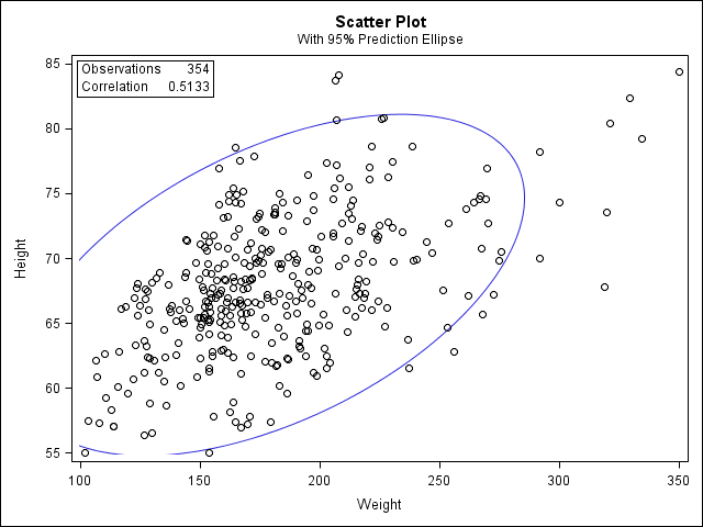
Before the Test

Before we look at the Pearson correlations, we should look at the scatterplots of our variables to get an idea of what to expect. In particular, we need to determine if it's reasonable to assume that our variables have linear relationships. PROC CORR automatically includes descriptive statistics (including mean, standard deviation, minimum, and maximum) for the input variables, and can optionally create scatterplots and/or scatterplot matrices. (Note that the plots require the ODS graphics system . If you are using SAS 9.3 or later, ODS is turned on by default.)

In the sample data, we will use two variables: “Height” and “Weight.” The variable “Height” is a continuous measure of height in inches and exhibits a range of values from 55.00 to 84.41. The variable “Weight” is a continuous measure of weight in pounds and exhibits a range of values from 101.71 to 350.07.

Running the Test

Sas program.

The first two tables tell us what variables were analyzed, and their descriptive statistics.

The third table contains the Pearson correlation coefficients and test results.

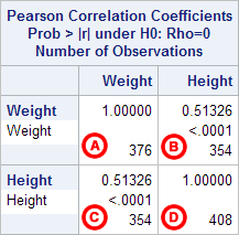
Notice that the correlations in the main diagonal (cells A and D) are all equal to 1. This is because a variable is always perfectly correlated with itself. Notice, however, that the sample sizes are different in cell A ( n =376) versus cell D ( n =408). This is because of missing data -- there are more missing observations for variable Weight than there are for variable Height, respectively.

The important cells we want to look at are either B or C. (Cells B and C are identical, because they include information about the same pair of variables.) Cells B and D contain the correlation coefficient itself, its p-value, and the number of complete pairwise observations that the calculation was based on.

In cell B (repeated in cell C), we can see that the Pearson correlation coefficient for height and weight is .513, which is significant ( p < .001 for a two-tailed test), based on 354 complete observations (i.e., cases with nonmissing values for both height and weight).

If you used the PLOTS=SCATTER option in the PROC CORR statement, you will see a scatter plot:

Decision and Conclusions

Based on the results, we can state the following:

• Weight and height have a statistically significant linear relationship ( r = 0.51, p < .001).
• The direction of the relationship is positive (i.e., height and weight are positively correlated), meaning that these variables tend to increase together (i.e., greater height is associated with greater weight).
• The magnitude, or strength, of the association is moderate (.3 < | r | < .5).
• << Previous: Analyzing Data
• Next: Chi-Square Test of Independence >>
• Last Updated: Dec 18, 2023 12:59 PM
• URL: https://libguides.library.kent.edu/SAS

Street Address

Mailing address, quick links.

• How Are We Doing?
• Student Jobs

Information

• Accessibility
• Emergency Information
• For Our Alumni
• For the Media
• Jobs & Employment
• Life at KSU
• Privacy Statement
• Technology Support
• Website Feedback

• How It Works

Pearson Correlation Coefficient

• July 4, 2021
• Posted by: admin
• Categories: SPSS Analysis Help, Statistical Test

Why is Pearson’s correlation used?

Pearson Correlation Coefficient is typically used to describe the strength of the linear relationship between two quantitative variables. Often, these two variables are designated X (predictor) and Y (outcome). Pearson’s r has values that range from −1.00 to +1.00. The sign of r provides information about the direction of the relationship between X and Y. A positive correlation indicates that as scores on X increase, scores on Y also tend to increase; a negative correlation indicates that as scores on X increase, scores on Y tend to decrease; and a correlation near 0 indicates that as scores on X increase, scores on Y neither increase nor decrease in a linear manner.

What does the Correlation coefficient tell you?

The absolute magnitude of Pearson’s r provides information about the strength of the linear association between scores on X and Y. For values of r close to 0, there is no linear association between X and Y. When r = +1.00, there is a perfect positive linear association; when r = −1.00, there is a perfect negative linear association. Intermediate values of r correspond to intermediate strength of the relationship. Figures 7.2 through 7.5 show examples of data for which the correlations are r = +.75, r = +.50, r = +.23, and r = .00.

Pearson’s r is a standardized or unit-free index of the strength of the linear relationship between two variables. No matter what units are used to express the scores on the X and Y variables, the possible values of Pearson’s r range from –1 (a perfect negative linear relationship) to +1 (a perfect positive linear relationship).

How do you explain correlation analysis?

Consider, for example, a correlation between height and weight. Height could be measured in inches, centimeters, or feet; weight could be measured in ounces, pounds, or kilograms. When we correlate scores on height and weight for a given sample of people, the correlation has the same value no matter which of these units are used to measure height and weight. This happens because the scores on X and Y are converted to z scores (i.e., they are converted to unit-free or standardized distances from their means) during the computation of Pearson’s r.

What is the null hypothesis for Pearson correlation?

A correlation coefficient may be tested to determine whether the coefficient significantly differs from zero. The value r is obtained on a sample. The value rho (ρ) is the population’s correlation coefficient. It is hoped that r closely approximates rho. The null and alternative hypotheses are as follows:

What are the assumptions for Pearson correlation?

The assumptions for the Pearson correlation coefficient are as follows: level of measurement, related pairs, absence of outliers, normality of variables, linearity, and homoscedasticity.

Linear Relationship

When using the Pearson correlation coefficient, it is assumed that the cluster of points is the best fit by a straight line.

Homoscedasticity

A second assumption of the correlation coefficient is that of homoscedasticity. This assumption is met if the distance from the points to the line is relatively equal all along the line.

If the normality assumption is violated, you can use the Spearmen Rho Correlation test

Our statisticians take it all in their stride and will produce the clever result you’re looking for.

Looking For a Statistician to Do Your Pearson Correlation Analysis?

9.1 Null and Alternative Hypotheses

The actual test begins by considering two hypotheses . They are called the null hypothesis and the alternative hypothesis . These hypotheses contain opposing viewpoints.

H 0 , the — null hypothesis: a statement of no difference between sample means or proportions or no difference between a sample mean or proportion and a population mean or proportion. In other words, the difference equals 0.

H a —, the alternative hypothesis: a claim about the population that is contradictory to H 0 and what we conclude when we reject H 0 .

Since the null and alternative hypotheses are contradictory, you must examine evidence to decide if you have enough evidence to reject the null hypothesis or not. The evidence is in the form of sample data.

After you have determined which hypothesis the sample supports, you make a decision. There are two options for a decision. They are reject H 0 if the sample information favors the alternative hypothesis or do not reject H 0 or decline to reject H 0 if the sample information is insufficient to reject the null hypothesis.

Mathematical Symbols Used in H 0 and H a :

H 0 always has a symbol with an equal in it. H a never has a symbol with an equal in it. The choice of symbol depends on the wording of the hypothesis test. However, be aware that many researchers use = in the null hypothesis, even with > or < as the symbol in the alternative hypothesis. This practice is acceptable because we only make the decision to reject or not reject the null hypothesis.

Example 9.1

H 0 : No more than 30 percent of the registered voters in Santa Clara County voted in the primary election. p ≤ 30 H a : More than 30 percent of the registered voters in Santa Clara County voted in the primary election. p > 30

A medical trial is conducted to test whether or not a new medicine reduces cholesterol by 25 percent. State the null and alternative hypotheses.

Example 9.2

We want to test whether the mean GPA of students in American colleges is different from 2.0 (out of 4.0). The null and alternative hypotheses are the following: H 0 : μ = 2.0 H a : μ ≠ 2.0

We want to test whether the mean height of eighth graders is 66 inches. State the null and alternative hypotheses. Fill in the correct symbol (=, ≠, ≥, <, ≤, >) for the null and alternative hypotheses.

• H 0 : μ __ 66
• H a : μ __ 66

Example 9.3

We want to test if college students take fewer than five years to graduate from college, on the average. The null and alternative hypotheses are the following: H 0 : μ ≥ 5 H a : μ < 5

We want to test if it takes fewer than 45 minutes to teach a lesson plan. State the null and alternative hypotheses. Fill in the correct symbol ( =, ≠, ≥, <, ≤, >) for the null and alternative hypotheses.

• H 0 : μ __ 45
• H a : μ __ 45

Example 9.4

An article on school standards stated that about half of all students in France, Germany, and Israel take advanced placement exams and a third of the students pass. The same article stated that 6.6 percent of U.S. students take advanced placement exams and 4.4 percent pass. Test if the percentage of U.S. students who take advanced placement exams is more than 6.6 percent. State the null and alternative hypotheses. H 0 : p ≤ 0.066 H a : p > 0.066

On a state driver’s test, about 40 percent pass the test on the first try. We want to test if more than 40 percent pass on the first try. Fill in the correct symbol (=, ≠, ≥, <, ≤, >) for the null and alternative hypotheses.

• H 0 : p __ 0.40
• H a : p __ 0.40

Collaborative Exercise

Bring to class a newspaper, some news magazines, and some internet articles. In groups, find articles from which your group can write null and alternative hypotheses. Discuss your hypotheses with the rest of the class.

As an Amazon Associate we earn from qualifying purchases.

This book may not be used in the training of large language models or otherwise be ingested into large language models or generative AI offerings without OpenStax's permission.

Want to cite, share, or modify this book? This book uses the Creative Commons Attribution License and you must attribute Texas Education Agency (TEA). The original material is available at: https://www.texasgateway.org/book/tea-statistics . Changes were made to the original material, including updates to art, structure, and other content updates.

Access for free at https://openstax.org/books/statistics/pages/1-introduction

• Authors: Barbara Illowsky, Susan Dean
• Publisher/website: OpenStax
• Book title: Statistics
• Publication date: Mar 27, 2020
• Location: Houston, Texas
• Book URL: https://openstax.org/books/statistics/pages/1-introduction
• Section URL: https://openstax.org/books/statistics/pages/9-1-null-and-alternative-hypotheses

© Jan 23, 2024 Texas Education Agency (TEA). The OpenStax name, OpenStax logo, OpenStax book covers, OpenStax CNX name, and OpenStax CNX logo are not subject to the Creative Commons license and may not be reproduced without the prior and express written consent of Rice University.

Hypothesis Testing with Pearson's r (Jump to: Lecture | Video )

Just like with other tests such as the z-test or ANOVA, we can conduct hypothesis testing using Pearson�s r.

To test if age and income are related, researchers collected the ages and yearly incomes of 10 individuals, shown below. Using alpha = 0.05, are they related?

1. Define Null and Alternative Hypotheses

2. State Alpha

alpha = 0.05

3. Calculate Degrees of Freedom

Where n is the number of subjects you have:

df = n - 2 = 10 � 2 = 8

4. State Decision Rule

Using our alpha level and degrees of freedom, we look up a critical value in the r-Table . We find a critical r of 0.632.

If r is greater than 0.632, reject the null hypothesis.

5. Calculate Test Statistic

We calculate r using the same method as we did in the previous lecture:

6. State Results

Reject the null hypothesis.

7. State Conclusion

There is a relationship between age and yearly income, r(8) = 0.99, p < 0.05

Back to Top

• school Campus Bookshelves
• menu_book Bookshelves
• perm_media Learning Objects
• login Login
• how_to_reg Request Instructor Account
• hub Instructor Commons
• Download Page (PDF)
• Download Full Book (PDF)
• Periodic Table
• Physics Constants
• Scientific Calculator
• Reference & Cite
• Tools expand_more
• Readability

selected template will load here

This action is not available.

14.8: Alternatives to Pearson's Correlation

• Last updated
• Save as PDF
• Page ID 22155

• Michelle Oja
• Taft College

The Pearson correlation coefficient is useful for a lot of things, but it does have shortcomings. One issue in particular stands out: what it actually measures is the strength of the linear relationship between two variables. In other words, what it gives you is a measure of the extent to which the data all tend to fall on a single, perfectly straight line. Often, this is a pretty good approximation to what we mean when we say “relationship”, and so the Pearson correlation is a good thing to calculation. Sometimes, it isn’t. In this section, Dr. Navarro and Dr. MO will be reviewing the correlational analysis you could use if you're a linear relationship isn't quite what you are looking for.

Spearman’s Rank Correlations

One very common situation where the Pearson correlation isn’t quite the right thing to use arises when an increase in one variable X really is reflected in an increase in another variable Y, but the nature of the relationship is more than linear (a straight line). An example of this might be the relationship between effort and reward when studying for an exam. If you put in zero effort (x-axis) into learning a subject, then you should expect a grade of 0% (y-axis). However, a little bit of effort will cause a massive improvement: just turning up to lectures means that you learn a fair bit, and if you just turn up to classes, and scribble a few things down so your grade might rise to 35%, all without a lot of effort. However, you just don’t get the same effect at the other end of the scale. As everyone knows, it takes a lot more effort to get a grade of 90% than it takes to get a grade of 55%. What this means is that, if I’ve got data looking at study effort and grades, there’s a pretty good chance that Pearson correlations will be misleading.

To illustrate, consider the data in Table \(\PageIndex{1}\), plotted in Figure \(\PageIndex{1}\), showing the relationship between hours worked and grade received for 10 students taking some class.

The curious thing about this highly fictitious data set is that increasing your effort always increases your grade. This produces a strong Pearson correlation of r=.91; the dashed line through the middle shows this linear relationship between the two variables. However, the interesting thing to note here is that there’s actually a perfect monotonic relationship between the two variables: in this example at least, increasing the hours worked always increases the grade received, as illustrated by the solid line.

If we run a standard Pearson correlation, it shows a strong relationship between hours worked and grade received (r(8) = 0.91, p < .05), but this doesn’t actually capture the observation that increasing hours worked always increases the grade. There’s a sense here in which we want to be able to say that the correlation is perfect but for a somewhat different notion of what a “relationship” is. What we’re looking for is something that captures the fact that there is a perfect ordinal relationship here. That is, if Student A works more hours than Student B, then we can guarantee that Student A will get the better grade than Student b. That’s not what a correlation of r=.91 says at all; Pearson's r says that there's strong, positive linear relationship; as one variable goes up, the other variable goes up. It doesn't say anything about how much each variable goes up.

How should we address this? Actually, it’s really easy: if we’re looking for ordinal relationships, all we have to do is treat the data as if it were ordinal scale! So, instead of measuring effort in terms of “hours worked”, lets rank all 10 of our students in order of hours worked. That is, the student who did the least work out of anyone (2 hours) so they get the lowest rank (rank = 1). The student who was the next most distracted, putting in only 6 hours of work in over the whole semester get the next lowest rank (rank = 2). Notice that Dr. Navarro is using “rank =1” to mean “low rank”. Sometimes in everyday language we talk about “rank = 1” to mean “top rank” rather than “bottom rank”. So be careful: you can rank “from smallest value to largest value” (i.e., small equals rank 1) or you can rank “from largest value to smallest value” (i.e., large equals rank 1). In this case, I’m ranking from smallest to largest, because that’s the default way that some statistical programs run things. But in real life, it’s really easy to forget which way you set things up, so you have to put a bit of effort into remembering!

Okay, so let’s have a look at our students when we rank them from worst to best in terms of effort and reward:

Hm. The rankings are identical . The student who put in the most effort got the best grade, the student with the least effort got the worst grade, etc. If we run a Pearson's correlation on the rankings, we get a perfect relationship: r(8) = 1.00, p<.05. What we’ve just re-invented is Spearman’s rank order correlation , usually denoted ρ or rho to distinguish it from the Pearson r. If we analyzed this data, we'd get a Spearman correlation of rho=1. We aren't going to get into the formulas for this one; if you have ranked or ordinal data, but you can find the formulas online or use statistical software.

For this data set, which analysis should you run? With such a small data set, it’s an open question as to which version better describes the actual relationship involved. Is it linear? Is it ordinal? We're not sure, but we can tell that increasing effort will never decrease your grade.

Phi Correlation (or Chi-Square)

As we’ve seen, Pearson's or Spearman's correlations workspretty well, and handles many of the situations that you might be interested in. One thing that many beginners find frustrating, however, is the fact that it’s not built to handle non-numeric variables. From a statistical perspective, this is perfectly sensible: Pearson and Spearman correlations are only designed to work for numeric variables

What should we do?!

As always, the answer depends on what kind of data you have. As we we’ve seen just in this chapter, if your data are purely qualitative (ratio or interval scales of measurement), then Pearson’s is perfect. If your data happens to be rankings or ordinal scale of measurement, then Spearman’s is the way to go. And if your data is purely qualitative, then Chi-Square is the way to go (which we’ll cover in depth in a few chapters).

But there’s one more cool variation of data that we haven’t talked about until now, and that’s called binary or dichotomous .

Look up “binary” or “dichotomous” to see what they mean.

The root of both words (bi- or di-) mean “two” but the Phi (sounds like “fee,” rhymes with “reality”) correlation actually uses two variables that only have two levels. You might be thinking, “That sounds like a 2x2 factorial design!” but the difference is that a 2x2 factorial design has two IVs, each with two levels, but also has a DV (the outcome variable that you measure and want to improve). The Phi correlation has one of the two variables as the DV and the DV only has two options, and one of the two variables in the IV and that IV only has two levels. Let’s see some example variables:

• Pass or Fail
• Pregnant or Not pregnant
• Urban or rural
• Conservative or Progressive

How does this work into IVs and DVs?

• Does tutor (tutored or not-tutored) affect passing (pass or fail)?
• Does caffeine (coffee or no-coffee) affect energy (sleepy or not-sleepy)?
• Does exercise (exercise or no-exercise) affect weight loss (lose 10+ pounds or do not lose 10+ pounds)?

Again, we are not going to get into the formula for this one, but it is a unique statistical analysis that is designed for very specific variables. So when you have two binary variables, the Phi correlation is exactly what you should be using!

Curvilinear Relationships

We have one more situation in which Pearson’s correlation isn’t quite right, and that’s when we expect a non-linear relationship. We’ve seen this in scatter plots that are U-shaped or reverse-U shaped (the section of the graphing chapter on scatterplots , the section of this chapter on correlation versus causation in graphs , and the section in this chapter on strength, direction, and linearity ) . In that section on correlation versus causation in graphs , we talked about how plants die if they don’t have enough water but also if they have too much water. There is not a linear relationship between water and plant growth, it is a curvilinear relationship. There are specific statistical analyses that look for specific curvilinear relationships (based on how curved it appears to be) that we aren’t going to get into here, but they are available on advanced statistical software programs.

The key thing to remember, other than that these analyses exist, is that looking at the graph is key to helping you know what kind of analysis to conduct.

Contributors and Attributions

• Danielle Navarro ( University of New South Wales )

Dr. MO ( Taft College )